Undersampling. Playing with Nyquist and Shannon.
This week, Digilent released the Zmod SDR, a new ZMOD module with SYZYGY interface intended for SDR projects. The features of this new Zmod include 2 RX channels with 14-bit resolution and an analog bandwidth from just 35 kHz to 470 MHz. The very interesting part of this Zmod is that it features the ADC AD9648. This ADC from Analog Devices has a maximum sampling rate of 125 Msps but, the Zmod SDR can read signals up to 470 Mhz, Were Nyquist and Shannon looking to the other side when this module was designed? has Digilent broken the famous Nyquist-Shannon theorem that says that to acquire a signal we need to sample at least twice of the signal we want to acquire? Can also Digilent break the speed of light? All of these questions, except the last one, have an explanation, undersampling.
Let’s take a look at what Nyquist-Shannon said about sampling. In an easy world, where all the signals are in base band, we would need all the frequency components of the signal we want to acquire to be always below the sampling frequency divided by two. This is very important because when we discretize a signal, an image signal is also present in the second half of the sampling frequency like in a mirror, so if our original signal reaches half of the sampling frequency, part of this image signal would be in the first half, producing aliasing. Until here, nothing new.

What your teacher may have forgotten to tell you is that the image signals generated when we discretize a signal, are repeated in all the frequency domain, from zero to infinite, and also from zero to -infinite. This effect will generate what is known as Nyquist Zones, which are the zones where the image signals are repeated.

As we said before, the image signal between fs/2 and fs is mirrored, but the image signal from fs to fs+fs/2 is not, so this image will have the same shape as the original one, which is very interesting. Generalizing this, we can say that, a signal that is located in the frequency range from 0 to fs/2, will be repeated every fs·n. In the same way, we can find the signal mirrored every fs/2+fs·n, being n positive and negative, and the negative ones are the key for undersampling.
Since the image signals are repeated in all the frequency spectrum, what happens if the original signal is located at the Nyquist Zone 5? Since it is an odd zone, the signal is not mirrored with respect to the first Nyquist Zone, so an image in the base band can also be read, an image with the same shape than the original. In other words, we can read in base band the same signal that, in reality, is located at a much higher frequency, isn’t it great?

To understand how it works, we need to be sure that the signal is periodic, so its shape does not change fast. Let’s see a very simple example, imagine that we have a signal with a frequency of 17x, being x any number, and we are acquiring at 8x. Indeed, we can not acquire several points from a cycle of the faster signal, but we are going to take a point from the first cycle, another point from the third, another from the fifth… and finally, with all those points, we will have a signal, with the same shape of the fast one, but translated in frequency. In this exact case, with a sampling frequency of 8x, the 17x signal is located at the fifth Nyquisq Zone. Since that zone starts in fs*2, which is 16x, and the original signal has a frequency of 17x, I will see a signal of 1x.

For a single harmonic signal seems obvious how it works, but for complex signals, although could seem complex, it is just the same. With the help of Matlab, we are going to generate a signal consisting of several harmonics with different amplitudes.
fs = 10e6;
t = 0:1/fs:0.01

fbase = 100e3;
signal =  0.5 * cos(2*pi*(fbase * 1.02)*t);
signal = signal + 0.1 * cos(2*pi*(fbase * 1.05)*t);
signal = signal + 0.2 * cos(2*pi*(fbase * 1.06)*t);
signal = signal + 0.4 * sin(2*pi*(fbase * 1.07)*t);
signal = signal + 0.1 * sin(2*pi*(fbase * 1.09)*t);
For this signal, I have supposed a sampling rate of 10 Mhz, but it will work with continuous signals too. The shape of the signal is the next.

Now we can calculate the DFT of the signal using the comman fft.
signalDft = abs(fft(signal))*2/length(signal);
fVector = linspace(0,fs - fs/length(signal),length(signal));
Here we can find the harmonics of the signal. In this case, we have harmonics in the range of 102 KHz to 109 kHz.

Ok, now, we are going to resample the signal. Notice that the bandwidth of the signal is 7 KHz (109 KHz - 102 kHz). In this case we are going to reserve a bandwidth of 10 kHz, so we need to acquire at least at 20kHz to avoid aliasing.
Matlab has a function called resample, but it performs in addition to the resample itself, a set of filters. For this example I preferred to perform the resample with a for loop, and increase the index the undersampling factor, that is, I am going to take just one sample every uFactor samples.
fs2 = 20e3;
t2 = 0:1/fs2:0.01-1/fs2
uFactor = fs/fs2;
USignal = [];

i = 1;
while i < length(signal)
    USignal = [USignal, signal(i)];
    i = i+uFactor;
end

At this point, the resampling is finished, no filtering is needed in this case. If we calculate again the DFT of the signal, we can see how the signal consists of the same harmonics, but shifted 100 kHz.
USignalDft = abs(fft(USignal))*2/length(USignal);
fUVector = linspace(0,fs2 - fs2/length(USignal),length(USignal));

This example has worked because we have selected an undersampling factor that allows capturing all the harmonic components of the signal, and this is very important. If you have a signal with harmonics in the whole spectrum, first you will need to filter to reduce all the harmonics out of the bandwidth desired.
Now we know that we can acquire signals of any frequency with a much less frequency, is something missing in this process? yes. This process is not free, and to know what will happen to the captured signal, we need to recover the Signal to Noise Ratio (SNR) equation.
The SNR is a measure of how well a system rejects noise. For an acquisition method, it is related to the number of bits of the signal (N), and two extra constants.
\[SNR=6.02N+1.76\]The result of this equation measures the uncertainty of the signal measured. If I have a 12-bit ADC, the amount of signal between one LSB and the next is 1/4096, however, if my ADC has 16 bits of resolution, the uncertainty is decreased to 1/65536. Okay, but where is the sampling rate in this equation? In the process gain. The original SNR equation can be completed with a third factor
\[SNR=6.02N+1.76+10 \cdot log_{10}\left( \frac{fs}{2BW} \right)\]In this blog we already saw this equation when we talked about oversampling, and the theory is the same. When we perform oversampling, which means capture the signal several times above the Nyquist frequency, the SNR increased, and the Equivalent Number of Bits (ENOB) increases. For this case is exactly the opposite, since the term fs is decreased, the SNR is also decreased.
To verify this, we can add some noise to the original signal.
fs = 10e6;
t = 0:1/fs:0.01

fbase = 100e3;
signal =  0.5 * cos(2*pi*(fbase * 1.02)*t);
signal = signal + 0.1 * cos(2*pi*(fbase * 1.05)*t);
signal = signal + 0.2 * cos(2*pi*(fbase * 1.06)*t);
signal = signal + 0.4 * sin(2*pi*(fbase * 1.07)*t);
signal = signal + 0.1 * sin(2*pi*(fbase * 1.09)*t);
signal = signal + 0.4*rand(1,length(signal));
We can see that the amplitude of the harmonics in the original signal barely has been modified.

However, once the signal is resampled, the error in the amplitude of the harmonics has been increased. In addition, we can see a noise floor.

The undersampling is a very useful technique that engineers have available to use, however it has to be used carefully. Although it can be used for communication, using it as a demodulator, is not the more common way to do it. Devices like the USRP B205mini-i, or the B210, also from Digilent, use an analog demodulation stage, that uses signal mixers to decrease the frequency of the signals, keeping the SNR. In any case, this board is a very interesting option to discover how we can process radio signals in FPGA.