Running subcycle average models on Speedgoat Performance System (I).
 Speedgoat
Materials like Silicon Carbide (SiC) or Gallium Nitride (GaN) are making our power electronics converters faster and faster. This means small inductors and capacitors that make, in most cases, the cost of the devices decrease. This also means that the control devices also have to be faster, and not only the microcontrollers or the digital signal processors but the simulation benches where these devices are tested against models also have to follow the materials allowing faster simulations. For small models running on FPGA this is not a big deal. FPGA are capable of running models very fast but when we have complex models, this task can turn complicated.
If we analyze what an FPGA has to do to simulate a power electronics model, the first is capturing the control signal, which in the 95% of cases is a PWM signal so, let’s start from the beginning.
PWM signal
A PWM signal seems a square signal with two big differences. The first one is that the PWM has an offset, which means that the lower value of the signal will be zero. On the other hand, in a square signal, the time that the signal value is one is half of the period, making that the average value of the signal, or the DC component of the signal will be amplitude divided by two. In a PWM signal, the time in which the signal value is high is different than the time in which the value of the signal is low, so the DC value of a PWM can be different than the amplitude divided by two. We can find that PWM signals are defined by their period \(T\), and their duty cycle which can be calculated as \(\frac{t_{on}}{T}\). Also we can define the \(t_{off}\) as \(T-t_{on}\).

If we analyze the PWM signal applying a DFT, we can find what we mentioned before, there is a DC value in the PWM that corresponds with the duty cycle (\(D\)) times the Amplitude (\(A\))
\[DC = D \cdot A\]Since the PWM signal is a kind of square wave, the DC component is not the only component we can find in the DFT. Like a square signal, the harmonic spectrum draws a \(sinc\) function starting in the base frequency. The asymmetry in the PWM signal has some effects on its frequency spectrum. In the next figure, we can find how the amplitude of the different harmonics changes according to the duty cycle of the signal. For example, for a duty cycle of 0,5 or 50%, we can see how the even harmonics are canceled, and the first harmonic is even greater than the DC value.

Now, that we know what is a PWM signal, the next is to learn how devices like the Speedgoat can capture that signal.
Capturing the PWM signal
Capturing a PWM signal is not different than capturing any other signal. We just need to “read” the input pin in order to know the state of the signal, and then execute the model with the read value. In addition, since the value of a PWM signal can be only ‘1’ or ‘0’, we just need a digital input to capture the signal, easy? Well, it depends.
While reading the digital input pin is a very easy task, an Arduino Nano can do it, calculating the effects of that value in the rest of the model can be very complex. In the next image, we can find three different PWM signals, all of them with the same duty cycle, so the DC value of each one is the same, but all three signals have different frequencies. In gray we can find the points where the PWM signal is captured with a frequency of \(fs\). If we don’t think in the model, we can see that for the first signal, the first harmonic is located at \(fs/16\). For the second one, the first harmonic is located at \(fs/8\), and for the third one is located at \(fs/4\). If we continue increasing the PWM frequency, the first effect we will find is aliasing, so images of high-power harmonics will appear near the DC value, distorting this value and making the signal unreadable.

Another effect that we may encounter if the sampling frequency is not far enough from the PWM frequency is related to the time step of the model. When the PWM signal is captured, the next step is calculating the next output of the model. According to the complexity of the model, the time spent in the calculation, the time step, could be so much, so the sampling frequency has to be reduced. If the sampling frequency is not reduced, we will find timing errors in the model since a new input is captured while the last output is not calculated yet. This effect may break the model and likely will stop the simulation. In the case that the time step of the model and the capture frequency will be so near, the entire model can be aliased, so the fidelity of the model will decrease, which can be an effect worse than the latest because this time, the model could seem working fine, but the results are far from the reality.
In any case, the fact that the PWM frequency and the time step of the model are close is a big problem. In order to fix this problem, we can apply the Subcycle Average technique. Let’s explain this.
Subcycle average
In a perfect world, the time step of a model would be zero. Since this is not a perfect world, this time is related to three different points.
- Complexity of the model.
- Speed of the device that has to execute the model.
- Performance of the solver.
The complexity of the model is a parameter that is (relatively) out of our hands. If we need to execute a Dual Active Bridge (DAB) model, we cannot change it by an RC filter model in order to make it simpler but is true that we can apply some modifications to the DAB model to make it easy to simulate. The second point is the speed of the device, which is obvious, if we can calculate the operations that describe the model quickly, we will be ready to read a new input sample before. Finally, the solver is the algorithm that generates the different equations from the model, so if the solver generates simpler equations to describe the same behavior, then the device will calculate these equations quickly, reducing the time step.
For the Speedgoat devices, the time step of the model can be calculated as follows.
\[Time Step = \frac{FPGA_{CLK}}{OversamplingFactor \cdot NSolverIterations}\]The FPGA clock is related to the second point while the other parameters are related to the solver and the complexity of the model. For a model and a device, the time step is given so, in principle, the PWM frequency is limited by the time step, but just in principle. There is a method that allows us to decouple the PWM frequency and the time step of the model. Let’s take a look at the next diagram.
We can see an external control that generates a PWM signal at 100 kHz. Then, we can see a Speedgoat with a CPU that executes its model with a time step of 50 us, and an FPGA that executes the model at 10us (\(tsm\)) but, there is a little part of the FPGA model named PWM capture that is executed ten times faster (\(ts\)). If you are familiar with FPGA development, you will notice that we can find two different clock domains, and in the same way that we need to use synchronizers to connect different clock domains, this time we need to do the same with the block name Rate Converter.

Focusing on the PWM capture module, it has to oversample the PWM signal to get an accurate value duty cycle. The oversampling factor we need to apply depends on the PWM resolution we need. The PWM resolution is the number of steps in which we split a PWM cycle, therefore the oversampling factor will be \(\frac{T_{PWM}}{PWM_{resolution}}\). The output of the PWM capture module will be a value between 0 and 1 that represents the duty cycle of the signal, and it will be computed at \(tsm\). In the next model you will find the Simulink model that implements the PWM capture module where the value of the duty cycle captured is PWM pu.

The above model essentially counts the samples at \(ts\) where the input signal value is ‘1’, and also the samples in which the PWM signal value is zero. To obtain a value in the range 0 to 1, we need to divide by the oversampling factor \(tsm/ts\). The output ton of this module, for a PWM of 70 kHz, and a duty cycle of 20% is the next.

We can find how the PWM pu signal takes values in the range 0 to 1, and it is updated at \(tsm\) rate. The average value of PWM pu signal is 0.2. Having a continuous signal instead of a PWM, as we can expect, makes it possible to lose some of the information but, in terms of control, the regulators and systems, in general, have a reduced bandwidth, so to simulate correctly the control loop, we just need to compute the model faster than the bandwidth of the system. In the next figure we can see that the output of the control loop is indeed a continuous signal, so the PWM is “just” a way to transmit that signal to the power stage.

At this point, we have converted the PWM signal into a continuous signal that represents the average value of the signal of interest, and this is very important because we need to know which is our signal of interest, which is related to the bandwidth of the regulator. If we are controlling a DC-DC converter, we know that both the input and the output are DC, so, in short, the output of the regulator will be also a DC, therefore the bandwidth needed is small. In an AC-DC converter, the input signal is moving, so the regulator has to be able to control this moving signal, in other words, the bandwidth of the regulator has to be enough for the input signal, and not just the regulator but the bandwidth of the path from the regulator to the converter has also to be able to manage that bandwidth. This bandwidth can be controlled in a subcycle average model with the time-step of the model and the capture block. To get more information about subcycle averaging MATLAB has some interesting content on its webpage. This video about “Improving Resolution for Real-time Simulation” provides some extra information about this topic.
In the next post, we will create and deploy a subcycle average model in the Speedgoat Performance using what we have learned in this post.