Getting started with Speedgoat.
 Speedgoat
On this blog we have seen many projects where we have used FPGA, in general using development boards, unfortunately, there are not many cases where I can show you an FPGA in a real application, but this is one of these cases. The device I am talking about is a Real-Time Target Machine from Speedgoat, a test machine able to run Simulink models in real time. The uses of these devices are many different, from using it to test a control algorithm designed on Simulink with the real hardware to control, up to using the device to run a physical model and interact with that model using external hardware, in order to test the control algorithm running on the final device. Because of my job, I have used a device similar to this to test the control algorithm of a grid inverter in different grid scenarios and is very interesting how this kind of devices can reproduce very accurately the physical model. The task of this device is “only” running the model, but the task of translating that model into a set of discrete equations belongs to MATLAB. In this article, we are going to see how we can use the device to read a signal, execute an algorithm over that signal and then output the resulting signal, and part of these tasks will be performed by an FPGA.
Speedgoat has several products in its catalog. We can find small devices like the Unit, where, in addition to a CPU, we only can connect one small expansion IO module, up to the customizable large devices where the number of IO modules can be as large as your application needs, and they can integrate multiple FPGA working in parallel. In my case, MathWorks has lent me the Baseline device, which can allocate inside up to 4 IO modules in its S variant.

The Baseline device is based on a quad-core Intel Celeron processor running at 2.0 GHz. The device runs the Simulink Real-Time Operating System which is very integrated with Simulink and MATLAB, and allows running models in real-time, with a user-configurable sampling time. As I mentioned before, this device can allocate up to 4 IO modules. Each of these modules is connected to a mPCIe socket with one lane. The device I have has 2 communication modules, and an IO module, which is the most interesting for us. The IO module is the IO397. This IO module is based on an Artix7 50t FPGA and adds to the device 4 analog inputs, 4 analog outputs and 14 digital IOs. The ADC that is mounted on the board is the LTC2348-16, a 16 bits bipolar ADC which is connected to the FPGA through an SPI bus. The DAC used in this module is the AD5754R, a 16 bits bipolar DAC with SPI interface.

Inside the device, the connection diagram would be as follows. We have an Ethernet connection that communicates the device with the host PC. This interface is managed by the CPU and is used to send the model designed in Simulink to the device, as well as to send real-time signals from the device to the host in order to store and plot them. The device runs at the same time the CPU and the FPGA, and make them work in a co-simulation mode, where part of the model is executed by the CPU and the rest is executed in the FPGA. The distribution of the model between the CPU and the FPGA is made on Simulink, and is completely configurable by the user. The CPU and the FPGAs of the different IO modules are communicated through a PCIe Gen2 interface.

To begin to use the device, first, we need to download some packages that have to be installed in MATLAB. First of all, in order to use the Speedgoat as a controller, we will need access to the IO397 ADC and DAC from the Simulink model. To access those peripherals we will need to use some Simulink blocks specifically for the IO397. We have to navigate to the Speedgoat webpage, introduce our user’s credentials and a link to download the Speedgoat I/O Blockset will be available. Notice that the blocks are designed for a particular version of MATLAB so you need to download the package for your MATLAB version. When the file is downloaded and unzipped, we need to execute from MATLAB command window the script speedgoat_setup, and the installation process will start.
>> speedgoat_setup


________________________________________________________________________________

                         Welcome to the installer of
                     Speedgoat I/O Blockset Version 9.5.1
                              for MATLAB R2022b
________________________________________________________________________________

Checking pre-requisites...
- Host OS:        Linux               OK
- MATLAB release: R2022b              OK
- Support Package: installed          OK
- Simulink Real-Time license:         OK
- Accept EULA:                        OK

Currently installed Speedgoat I/O Blockset: v9.5.1 29065 (15-Dec-2022 17:06:07)
Would you like to uninstall it, and install v9.5.1 now? [y]/n : y

There are open Simulink systems! Save your system otherwise all unsaved changes are lost. Continue? [y]/n : y

Uninstall complete: 100%
Copying common files...
Copying block library files...
Copying product examples...
Installing mex files...
Refreshing Simulink Library Browser. This might take some time...


The Speedgoat I/O Blockset has been successfully installed.
Type "speedgoat" in the MATLAB Command Window to get started.
In addition to the blockset, we have to install the IO397 Configuration package, also available on the Speedgoat webpage. When the zip file is downloaded, we can install it running the script io_configuration_package_installer from the MATLAB command window.
>> io_configuration_package_installer
 => Do you want to install the Speedgoat IO397 Configuration Package? [y]/n: y

There are open Simulink systems!
Save your system otherwise all unsaved changes are lost. Continue? [y]/n : y
OK
 - Installing: io397_sources_v4.1: OK
 - Rehashing toolbox: OK
Speedgoat IO397 Configuration Package successfully installed.
>>
Now, we can connect the device and check the connections. The Speedgoat is connected to the host PC through an Ethernet connection. The IP of the device is static, although it can be changed once the connection is established. When the device is physically connected to the host pc, we can send a ping request to verify that the connection is active. Also, it is possible to connect the Speedgoat to a private network and access remotely upon configuring the gateway accordingly.
pablo@friday:~$ ping 172.16.107.5
PING 172.16.107.5 (172.16.107.5) 56(84) bytes of data.
64 bytes from 172.16.107.5: icmp_seq=1 ttl=255 time=0.185 ms
64 bytes from 172.16.107.5: icmp_seq=2 ttl=255 time=0.153 ms
64 bytes from 172.16.107.5: icmp_seq=3 ttl=255 time=0.152 ms
64 bytes from 172.16.107.5: icmp_seq=4 ttl=255 time=0.160 ms
64 bytes from 172.16.107.5: icmp_seq=5 ttl=255 time=0.164 ms
64 bytes from 172.16.107.5: icmp_seq=6 ttl=255 time=0.168 ms
64 bytes from 172.16.107.5: icmp_seq=7 ttl=255 time=0.153 ms
^C
--- 172.16.107.5 ping statistics ---
7 packets transmitted, 7 received, 0% packet loss, time 6123ms
rtt min/avg/max/mdev = 0.152/0.162/0.185/0.010 ms
Then, if the device responds correctly, we can establish the connection using MATLAB and the command slrtExplorer.
>> slrtExplorer
Simulink Real-Time Explorer is the tool in which we can manage real-time devices. Actions like connecting, changing IP address, updating the hardware of the device or rebooting it are the actions we can execute from this tool. When we connect the Speedgoat by clicking on the top-left of the window, we will see the internal disk usage of the device as well as the models that are loaded into the internal memory.

At this point, we have the Speedgoat connected to MATLAB, so we can start to develop for it. In this article, as we mentioned before, we are going to use the Speedgoat as a controller, that is, we are going to use the IO397 to read an external signal, that signal will be sent through the PCIe bus to the Speedgoat CPU, and this will execute an algorithm. Then, the output of the algorithm will be sent again through the PCIe bus to the IO397, and it will generate the corresponding signal. Since the design will be based on a Simulink model, the first we have to do is open Simulink by executing simulink in the command window.
When the Simulink window is opened, we need to select a Blank model, and a clean model will be opened. On this model we need to include the blocks needed to communicate the model with the IO397, and also the corresponding blocks to manage the IO ports, either analog or digital.
The block that will allow the communication between the CPU and the IO397 through the PCIe bus is a block named IO3xx setup. This block can be found on the Simulink library Simulink Real-Time: Speedgoat I/O Blockset > IO3xx > Setup.

When this block is added to the model, we can configure it. First of all we need to configure the exact module that we have inside our device since this block is used for several modules. In this case, the module is IO397-50k. Then, the block allows having connected several modules, each one identified by a Module ID. Thi Module ID is needed because you may have multiple modules of the same type. Since we only have one module, the Module ID is 1. The next configuration is the Configuration File or Bitstream. Remember that the IO397 is based on an Artix7 FPGA, so we need a configuration file loaded in the FPGA. Speedgoat gives us three different bitstreams for this module, one to use the module as Hardware-In-the-Loop (HIL), another one to use the module as Rapid-Control-Prototyping (RCP) or the last one, as a Communications device. According to the bitstream selected, in .mat format, the Pin Mapping of the device will change. To test the capabilities and as a first approach to this device, we are going to use the Speedgoat to generate a simple sine signal. To generate a signal, we are going to use just the DAC, so all the digital IO will remain unconnected. When you try to change the Configuration File, you will notice that the Pin Mapping that changes according to the configuration is the one of the digital IO, changing from pulse capture (PWM and Encoder) when the HIL is selected, to PWM generation when the RCP is selected. Since we will use just the DAC, we can select any configuration. now, we already have the Setup block configured, the next is configuring the Analog Outputs.
To manage and configure the Analog Outputs we need to add to the model the corresponding block, which can be found in the Simulink library Simulink Real-Time: Speedgoat I/O Blockset > IO3xx > Analog IO > IO397 Analog Output.
The configuration of this block is very simple. We only have to configure the output port as a vector, the initial values and the sampling time. Finally, we can configure the output range of the signal.

The sampling time selected in the IO397 Analog Output block, is the sampling time at which the CPU will send a new value to the DAC, but remember that the DAC used by the IO397 has a maximum sampling frequency of 200 ksps, that is a sampling period of 5e-6s, so the signal generated by the device will be sampled at the DAC sampling time.
At this point, the only element missing in the model is the sine signal generator.

Once we have our model complete, we need to convert our regular model to a real-time model, and this is done by executing the Simulink Real-Time app.

This application will change several parameters of the model in a single action in order to make it executable in real-time as well as change the solver to use a real-time solver.

Now we just click on the Run on Target* button, and Simulink will generate the C++ code of the model, compile and deploy it on the Speedgoat.

To know which pins are connected to the DAC, we can check the Speedgoat IO397 Hardware Reference Manual available in the Downloads section of your Speedgoat account.

In order to check the real-time step at which the CPU of the device is executing the model, we can click on the bottom-right of the window. Remember also that the model has to be configured to finish at the time inf to keep the model running forever.

If we want to generate a PWM instead of an analog signal, to active an IGBT for example, we need to change the Configuration File from HIL to RCP. Opening in this case the Pin Mapping we will see that the PWM signals are available now on the Digital IO ports.

To manage the PWM signal generation, on the model we need to add a block to generate the signals. That block is located in the library Simulink Real-Time: Speedgoat I/O Blockset > IO3xx > PWM > PWM generation (5). This block, unlike the Analog Output block, this time we will find many different configurations. For the sake of this example, we are going to generate a simple PWM signal, configuring 2 negated channels, with a dead band of 10 microseconds and a period of 0.1 milliseconds. The value of these parameters will depend on the FPGA frequency that can be found in the Setup block.

The input of the PWM Generation v5 block will be an analog signal with an amplitude that will configure the duty cycle of the signal.

Following the same steps to deploy the model in the device, we will see the PWM signal generated.

And the configured dead time.

Now that we already have seen how the device works, we are going to deploy a real application. The application although is simple, will allow us to use the CPU of the Speedgoat to execute an algorithm, a Band-Reject Low-Pass Filter. This kind of filters have a frequency response like the shown in the below diagram.

We can see that the initial response is a low-pass filter with gain, but later have a notch at the configured frequency. The MATLAB script to calculate the coefficients are the next.
%% Filter definition

s = tf('s'); % s variable deifnition

% notch frequency
fn = 1000;
wn = 2*pi*fn;

% low-pass frequency
fnlp = 500;
wnlp = 2*pi*fnlp;

% quality factor
q = 2;

% transfer function
h = (s^2+wn^2)/(s^2+wnlp/q*s+wnlp^2);

% draw bode diagram
bode(h)
To read and write the signals, we are going to use the analog Output and Analog inputs blocks from the Speedgoat library.

Then, the model of the filter will be a level above the hardware management.

Using the continuous model of the filter means that Simulink will create the real-time model of the filter using the real-time solver. If we need to control more precisely the digital implementation of the filter using the bilinear or any other discretization method, we can use a discretized model of the filter instead.
The next steps are known, we need to deploy the model into the Speedgoat, and by generating a frequency sweep signal with the Digilent ADP5250, we can read from Simulink the response of the filter.

Let’s analyze what is happening here. The analog signal generated by the ADP5250 is read by the ADC of the IO397 (shown in green). The signal is sent from the Artix7, using its PCIe interface to the quad-core Celeron processor of the Speedgoat Baseline, and the filter is calculated into the CPU within the sampling time configured (shown in blue). Then, the CPU sends through the PCIe bus the output signal of the filter, and the FPGA sends the signal to the DAC. In addition, the CPU sends through the Ethernet connection the signals to be plotted on Simulink.
In this article, we have used the Speedgoat device as a controller, reading an input signal, and executing an action according to the algorithm configured inside, but this is not the only way to use this device, actually, for me, this is the boring way. The most interesting way to use this device is by making it run as a hardware model. We can implement into the FPGA a discretized hardware model of, for example, an AC motor, and then use an external hardware to control that model, we can control the speed or the torque. In this case, model variables like current can be output through the analog output to be read for the external ADC and the speed can be translated into a train of pulses simulating an encoder, isn’t great? We will explore this application soon. Stay connected!