Frequency warping using the bilinear transform.
 Eclypse Z7
The process to design a IIR filter is always the same. First of all we have to design the design the filter using its continuous transfer function, then, once the natural frequency of the filter, the order and the quality factor are selected, we will obtain the corresponding s function. The next step in order to digitalize that filter, is apply some transformations to replace the variable s by z, this process is known as discretization. In order to discretize the continous transfer function we can use several methods, and one of the easy to use methods is Tustin, or the bilinear transform.
The bilinear transform is based on replace the \(s\) variable in the continuous transfer function by a function of z, but in this process, which is actually an approximation, we are going to introduce some errors. The size of that errors are related to the sampling frequency since a very (very very) high sampling frequency, in some cases, could seem continuous. In real systems, where the sampling frequency depends of the ADC and many real components, we can use high sampling frequencies, but in most cases we will introduce a significantly error. In case of the bilinear transform, the most important error that we will introduce is the frequency warping. This effect produces a shift of the natural frequency of the filter. This effect may be negligible in the case of a low pass filter, but in case of narrow band filters, the error could make that the filter didn.t work.
In order to find the error caused by the bilinear transformation, we need to find the relation between the analog frequency and the discrete frequency . First of all, we will start with the equation of the bilinear transformation.
\[s=\frac{2}{ts}\left(\frac{1-z^{-1}}{1+z^{-1}}\right)\]Replacing \(z\) by its polar form \(e^{j \omega d}\), we have
\[s=\frac{2}{ts}\left (\frac{1-e^{-j \omega d}}{1+e^{-j \omega d}}\right)\]Now, we are going to split the exponential using the half-angle.
\[1-e^{-j \omega d} = e^{-j \omega d/2} (e^{j \omega d/2}-e^{-j \omega d/2}) = e^{-j \omega d/2} \cdot 2j sin(\omega d/2)\] \[1+e^{-j \omega d} = e^{-j \omega d/2} (e^{j \omega d/2}+e^{-j \omega d/2}) = e^{-j \omega d/2} \cdot 2 cos(\omega d/2)\]Replacing in the above equation for the numerator and the denominator, we have:
\[s=\frac{2}{ts}\left ( \frac{e^{-j \omega d/2} \cdot 2j sin(\omega d/2)}{e^{-j \omega d/2} \cdot 2 cos(\omega d/2)}\right) = \frac{2j}{ts}\cdot tan(\omega d /2)\]Then, we have to find the relation with the analog , so we are going to equal both equations
\[\sigma + \omega a j = \frac{2j}{ts}\cdot tan(\omega d /2)\]We can verify that the real part is 0, and the imaginary part, witch \(\omega a\) is directly
\[\omega a = \frac{2}{ts}\cdot tan(\omega d /2)\]Notice that the limit when \(t_S\) tends to zero, is \(\omega a = \omega d\).
In MATLAB, we can check this deviation easily. First we have to declare a continuous band-stop filter. And the discretize the filter using the Tustin method.
close all
clear all
clc

% define filter
fc = 3000;
wc = 2*pi*fc;
q = 5;%1/sqrt(2); % butterworth

s = tf('s');

h = (s^2+wc^2)/(s^2+wc/q*s+wc^2)

%bode(h)

% discretize filter
fs = 100e6/2048
ts = 1/fs;

hz = c2d(h,ts,'tustin');

We can see how the frequency of the digital filter is moved. Then we will apply the pre-warping to the natural frequency, and re discretize the filter using this new frequency.
% calculate prewarping
wp = 2/ts*tan(wc*ts/2);
hw = (s^2+wp^2)/(s^2+wp/q*s+wp^2)
hwz = c2d(hw,ts,'tustin');

We can se how in this case, both frequencies are the same, so the error is fixed.
In order to verify that this effect occurs, and it is fixed using pre-warping, I am going to use the Digilent’s Eclypse Z7 with the ZMOD Scope and the ZMOD AWG. Also, to generate the signal and verify the response of the filter I am going to use the brand new Analog Discovery PRO 5250, witch has a signal 125 Msps signal generator as well as a two channels scope capable to acquire up to 1 Gsps.

To obtain the natural discretized frequency (\(\omega d\)), I am going to use a very useful function of the ADP 5250, which performs a frequency sweep obtaining for each frequency the gain of the filter, so the result will be the bode diagram of the filter. To configure this mode, we need to open the tool Network.

Once this tool is opened, we need to configure the number of points, and the minimum and maximum frequency. Also we need to configure the amplitude of the signal that the generator will generate. In this case, the natural frequency of my filter is 3 kHz, so the configuration I will use if 1V of amplitude, and a frequency range from 500 Hz to 10 kHz. The number of points will configure the frequency step. In my case, I have changed the number of points according to my needs.
First, I have configured the biquad filter as a band-stop butterworth filter, with a natural frequency of 3 kHz. This time I have not correct the frequency warp. Then, clicking on Single, the ADC 5250 will execute one entire swap. The result is shown in the next figure.

You can see how the response of the filter is the expected, but the natural frequency is 2.9407 khz, which is 59.3 Hz below the expected frequency. Applying the pre-warping to the frequency, the response of the filter is the next (notice that the zoom of the image is different).

With the frequency correction, the error if 0.0052 Hz, which is a despicable error. In the next test I have increased the quality factor of the filter to 5. This will have effect in the bandwidth of the notch, obtaining a narrower band filter.

The bilinear transformation is widely used to design IIR filters because its simplicity. We only have to replace s in the continuous transfer function by the z function. Other methods like impulse invariance needs of the partial fraction expansion algebra, so the process is a bit more complicated. Also, the bilinear transformation maps the entire s-plane, so there is no aliasing errors. On the other side, it produces a warping in the frequency, but using pre-warping, as we have seen in this post, we can fix that frequency deviation.
This is the first post where I have used the new Analog Discovery PRO 5250 and the results have been great. In the same tool we have an oscillosope (1 Gsps 8 bits), signal generator (125 Msps 14 bits), logic analyzer (16 inputs, 1 Gsps), and also digital IOs and a Digital Multimeter. In my case, this summer I will move to other place for 3 month, so we only need to take the ADC5250 and my laptop. The only con that I have encountered is that ADP5250 is not compatible (for now), with Linux, so I have to use it through a virtual machine running Windows since I use Ubuntu. In any case, I am thinking in some interesting posts using this tool.