Implementing a digital biquad filter in Verilog.
Filtering is likely the most common DSP algorithm that any embedded engineer has to design, no matter if they are developing for an STM32, TI DSP or, of course, an FPGA. Filtering is important because the majority of the applications are connected to the real world, so they need to capture real signals with the undesirable elements that all real signals have, i.e noise, offset… Also, signals that we need to acquire, not always will be the dominant signals we acquire, for example, for biological signals, we will acquire a high level of 50 or 60 Hz corresponding with the grid frequency. In this case, we will need a filter.
As you surely know as a reader of this blog, on digital systems, we have 2 kinds of filters, FIR (Finite Impulse Response) filter, which only uses the value of the input now and the value in the past, and IIR (Infinite Impulse Response), which use the value of the input now and in the past, and also the value of the past outputs. FIR filters are easy to design for many applications, on this blog we did that here, but the response is limited for low-order filters. On the other hand, with IIR filters, we can achieve more aggressive responses, but they have the disadvantage that the filter can be unstable in certain cases. On this blog, we already designed IIR filters here, but on that post, we used MATLAB to design the filter and HDL Coder to implement that filter. In this post, I will show how we can implement a second-order filter, or second-order system, on Verilog step by step.
Why a second order system?
Second-order systems are one of the 2 systems with which we can model any linear system. The other ones are the first-order systems. The reason is that if we want to create a third-order system, we can implement this system as a first-order system in series with a second-order system. In case we would to develop a 7th-order filter, we will generate 3 second-order filters in series with one first-order filter.
For example, a 5th-order system looks like the next equation.
\[H(s)= \frac{b0 + b1 \cdot z^{-1} + b2 \cdot z^{-2} + b3 \cdot z^{-3} + b4 \cdot z^{-4} + b5 \cdot z^{-5}}{1 + a1 \cdot z^{-1} + a2 \cdot z^{-2} + a3 \cdot z^{-3} + a4 \cdot z^{-4} + a5 \cdot z^{-5}}\]We can rewrite this equation as two 2nd order systems in series with a first-order system
\[H(s)= \frac{b01 + b11 \cdot z^{-1} + b21 \cdot z^{-2}}{1 + a11 \cdot z^{-1} + a21 \cdot z^{-2}} \cdot \frac{b02 + b12 \cdot z^{-1} + b22 \cdot z^{-2}}{1 + a12 \cdot z^{-1} + a22 \cdot z^{-2}} \cdot \frac{b01 + b11 \cdot z^{-1}}{1 + a11 \cdot z^{-1}}\]This kind of decomposition system is known as sections, and for the decomposition of second-order systems, we can find it on the internet and in literature as second order sections. Actually, in the post where I talk about the bandpass filter designed on MATLAB, the final implementation of the 8th order filter was four 2nd order filters in series (4 sections). On MATLAB command window, you can use the command tf2sos to convert a high-order filter into a set of second-order filters. In case you don’t have a MATLAB license, the Python library Scipy has the command scipy.signal.tf2sos, which performs the same function. Besides the improvement in simplicity that second-order filters allow us to achieve, when we are using a fixed-point encoding, implementing high-order filters can bring us stability issues, so splitting the filter in second-order systems will improve the stability of the system.
Verilog implementation.
Before starting coding, we have to think about what we want for the module we will create. In my case, is very important to be able to parametrize the module, this way, in case I change the width of the input, or the width of the output, that only represents a change on a parameter, without modifying the code of the module since it means new tests for the module. Also, we have to think about what numeric format we will use. For this kind of filter, is obvious that we will need a signed format, and the capability to manage decimal numbers. To achieve these requirements, we have to select between fixed point and floating point, and for me the decision is clear, I want a code that can be instantiated alone, without an external floating point unit, so the format will be fixed point. If we add the requirement of parameters, and the fixed point format, we will need parameters to define the width of the signals, and also the width of the decimal part, which will be related to the precision we need. Also, the precision will be selected to obtain a response of the implemented filter as similar as possible to the design. Now, how many widths do we need to parametrize? We can define one width that will be used for inputs and outputs and coefficients, but this way, the width of the coefficients will be selected according to the width of the data generator, and for some filters, which the coefficients are on the stability limit, this could represent a problem. So, at least we will define 2 different widths, one for the input and outputs, according to the data drain and the data source, and the other one according to the resolution we will need. Another thing we have to think about widths is the resolution of the internal operations because in some cases, a stability problem is not related to the width of the coefficient itself, but the operation resolution, so at this point, will be interesting decoupling the width of the coefficients that will be generated on MATLAB or Python, with the width of the internal filter operations. Finally, filter parameters will look like the next.
parameter inout_width = 16,
parameter inout_decimal_width = 15,
parameter coefficient_width = 16,
parameter coefficient_decimal_width = 15,
parameter internal_width = 16,
parameter internal_decimal_width = 15
Next, we have to think on the interfaces. For applications where data is transferred between modules in a continuous way, AXI4-Stream will be the best option. On the inputs and output field, we will define both master and slave AXI4-Stream interfaces to acquire and send data. Although the input and output widths are parametrize, if we want to connect the module to an existing AXI4-Stream IP, this width are restricted to the width of the bus.
input aclk,
input resetn,

/* slave axis interface */
input [inout_width-1:0] s_axis_tdata,
input s_axis_tlast,
input s_axis_tvalid,
output s_axis_tready,

/* master axis interface */
output reg [inout_width-1:0] m_axis_tdata,
output reg m_axis_tlast,
output reg m_axis_tvalid,
input m_axis_tready,
Regarding the coefficients, the best to insert them is with an AXI4-LIte interface, but I want to design this module without the need of using a Zynq or Microblaze, so the easy way to insert the coefficients is as inputs.
/* coefficients */
input signed [pw_coefficient_width-1:0] b0,
input signed [pw_coefficient_width-1:0] b1,
input signed [pw_coefficient_width-1:0] b2,
input signed [pw_coefficient_width-1:0] a1,
input signed [pw_coefficient_width-1:0] a2
Now, with all the inputs and outputs defined, we have to think about the data flow. First, as we have different formats defined, to be able to operate on the coefficients and data, we have to change the format of all signals to the internal format, which is defined by the internal width and the decimal width. The integer width used is defined as a localparam, and is corresponding to the difference between the width and the decimal width. To change the format, we will fill with zeros the low side of the signal until the decimal part will be completed. For the integer part, as the format used is signed, we have to perform a sign extension, that is filled with the value of the MSb until the integer part will be completed. Notice that this works because the internal width is bigger or equal to the inout and coefficients width. Digital filters, both FIR and IIR, need to store the value of the past inputs, and IIR also the value of the past outputs, so we will need a pipeline structure to store the past values.
/* pipeline registers */
always @(posedge aclk)
  if (!resetn) begin
    input_pipe1 <= 0;
    input_pipe2 <= 0;
    output_pipe1 <= 0;
    output_pipe2 <= 0;
  end
  else
    if (s_axis_tvalid) begin
      input_pipe1 <= input_int;
      input_pipe2 <= input_pipe1;
      output_pipe1 <= output_int;
      output_pipe2 <= output_pipe1;
    end
Now, the next is to perform the filter calculations. a second-order filter needs to perform 5 multiplications, and remember that it does not necessarily mean that the modules use 5 DSP slices. The code I developed performs combinational multiplications. This allows 0 clock cycles delay, but limits the speed of the filter. If your timing constraints are not met, you can register the input of the multipliers, and then make a retiming to let Vivado select where is more efficient to put the register.
/* combinational multiplications */
assign input_b0 = input_int * b0_int;
assign input_b1 = input_pipe1 * b1_int;
assign input_b2 = input_pipe2 * b2_int;
assign output_a1 = output_pipe1 * a1_int;
assign output_a2 = output_pipe2 * a2_int;
The result of the multiplications will be added, in case of the input, and substracted in the case of the outputs, to obtain the filter output. As the output of the product has a size of twice of the operands, the addition must be the same width. To use the output on the multiplications, we have to perform a shift to delete extra decimal positions. Regarding the extra integer position will be truncated on the assignment.
assign output_2int = input_b0 + input_b1 + input_b2 - output_a1 - output_a2;
assign output_int = output_2int >>> (internal_decimal_width);
Finally, the value of the output will be reformatted to the inout widths.
assign m_axis_tdata = output_int >>> (internal_decimal_width-inout_decimal_width);
Regarding the AXI4-Stream management signals, as the filter behaves as bridge, with one cycle delay, management signals will pass through the filter with one cycle delay.
Once the system is implemented we can test it.
Module verifying.
In order to verify the behavior of the filter, we will configure the system as a low pass filter, with a cut frequency of 1kHz, and a sampling frequency of 100kHz (script lowpass_sos.m). Then, we perform a unitary step to the filter. To obtain the response of the implemented filter, we configure the coefficients with a format of 20 bits and 18 decimal bits. The internal width will be the same as the coefficients. In MATLAB, also we can test the response of the quantized filter. Testbench used (axis_biquad_tb.v), logs the output data at a sampling frequency, so the output of both MATLAB and XSIM must be identical, with a gain of 1000 in the case of the simulation. The first response is made with an internal format of I2Q18, and we can see how the gain in DC is been attenuated. This is due to the resolution of the internal operations since MATLAB performs the operations with a resolution of 32 bits.

Now, with the same resolution of the coefficients, we will change the internal width to 32 bits, with 30 bits on the decimal side, and we obtain a response identical to the one obtained on the MATLAB model.

Configuring again an internal width of I2Q18, we can se how increasing the Q factor, the response of the filter remains stable and with an acceptable gain.

The use of a higher or lower resolution will depend on the application. The fact of using the double of multiplicators to achieve a DC gain almost the same as the continuous model will depend of the number of DSP Slices available on the part you are using, but in most cases, applying a gain to the transfer function of the filter will be enough. Another option would be use a lower number of multiplicators than multiplications, and use a pipeline to perform the operations. This option will be valid if the clock cycles between data valid signals are enough to perform all the operations. This technique is known as folding, and the factor between the number of operations and multiplications is named the folding factor.
One important thing about this post is that we have implemented a generic second-order system, that can be used as a filter, or as a regulator, or even a plant model to simulate a plant behavior on an FPGA. This kind of system is powerful and sure on a future post we will use this module to create some cool projects.