Adding windows to xFFT IP.
Digital signal processing algorithms are, in general, purely mathematical algorithms that works perfectly on our notebook or MATLAB, but in real design, the algorithm starts to return us some unexpected results. One example of that is the quantification error. While in MATLAB we have a floating point format with the double resolution, in our FPGA, in the major of the cases, we will have a fixed point with less than 64 bits of resolution. Other cases where the real world hits us with reality, is when we want to perform a DFT of FFT. In this case, we need to acquire a real signal with an ADC, and then send this samples to the DFT module. For example, imagine you have a module that performs a DFT of 16 samples, each one acquired at 500 Ksps. The first harmonic is corresponding with 500e3/16 = 31.25ksps, therefore if we acquire a signal of this frequency, the result will be as follows.
The phase of the acquired signal will not produce any distortion in the frequency analysis, only will provoke that the angle of the signal will be shifted. The resulting DFT of this signal is the next.
As we can expect, the DFT of a cosine signal is corresponding with only one value different than 0 on the frequency domain. The DFT works as expected. In a real system, this means that the signal that the ADC is acquiring has exactly 31.25kHz. The second harmonic of our sampled signal is corresponding with 62.5 kHz, and the DFT of this new signal is the next.
We can see how the DFT of this signal is, as expected, a single non-zero value on the DFT, but, what happens with all the frequencies between 31.25 kHz and 62.5 kHz? All the signals between the two harmonics of the DFT will be distributed in the entire bandwidth of our system. This effect is known as DFT leak, and we can check it in the next figures.
This signal has a frequency greater than the first harmonic but lower than the second, and we can see how in the frequency domain not only the first and the second harmonic are affected, but the spectrum has unexpected values. Without going into greater detail, this effect comes from the unsynchronized sinc signals of the DFT process. This can be checked easily if we increase the points of the DFT by adding zeros at the end of the signal, in order to increase the points of the DFT.
If we need to perform a frequency analysis of the signal, DFT leak can be a problem because it shows frequencies that are not in our signal, and there is no need to filter them. At this point, we need a technique that allows us to minimize this effect, and let us to know the real frequency content of our signal. This technique is known as windowing.
Windowing consists on apply to the acquired signal a mask that reduces the effect of the lateral samples, keeping the frequency spectrum. There are different kinds of windows, each one computed differently, but for the goal of this post, we only need to know that they can be computed in Python with the Scipy package, and obviously in MATLAB. In this example, I will use a Hamming window, and we can see how by multiplying the 16 points of the signals by the 16 points of the window, the frequency spectrum will be reduced on the frequencies far from the frequency of the signal.
On the other side, we can see an undesirable effect, the amplitude of the main harmonic has been decreased. This, in general, is not a big deal because the goal of the DFT in most cases is not to know the exact amplitude of the harmonics, but their position.
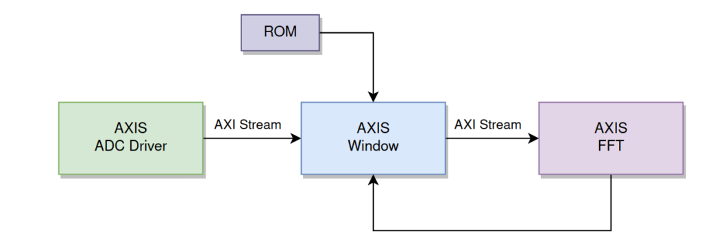
Unlike the window applied to the FIR filter coefficients, these coefficients must be applied in real-time, so to use this technique in the FPGA, we need to design a module in charge to apply the window to the read samples. This module will be located between the ADC driver and the xFFT module. The module needs to know the coefficients of the window to apply. In my design, these coefficients are stored in a BRAM module, initialized with a .coe file. Also, as the xFFT needs some time to compute the whole spectrum, we will need some control input to start the process. This signal will come from the xFFT module.
With all this information, we can define the inputs and outputs of the module.
module axis_window_v1_0 #(
  parameter window_length = 32,
  parameter inout_width = 16,
  parameter inout_decimal_width = 15,
  parameter window_coeff_width = 16,
  parameter window_coeff_decimal_width = 15,
  parameter internal_width = 16,
  parameter internal_decimal_width = 15,
  parameter memory_depth_width = 6
  )(
  input aclk,
  input resetn,

  input start_burst, /* start to apply window */

  /* slave axis interface */
  input [inout_width-1:0] s_axis_tdata,
  input s_axis_tlast,
  input s_axis_tvalid,
  output s_axis_tready,

  /* master axis interface */
  output [31:0] m_axis_tdata, /* fixed width for up to 16 bit xfft */
  output reg m_axis_tlast,
  output reg m_axis_tvalid,
  input m_axis_tready,

  /* window memory interface */
  output reg [memory_depth_width-1:0] mem_addr,
  input [window_coeff_width-1:0] mem_din
);
Now, as I always do with modules that perform mathematical operations, we need to transform the input signals to the internal width. In this case, the input signals will be the memory input, and the data input.
/* resize signals to internal width */
assign input_int = { {(internal_integer_width-inout_integer_width){s_axis_tdata[inout_width-1]} },
                            s_axis_tdata,
                            {(internal_decimal_width-inout_decimal_width){1'b0} } };
assign window_coeff = { {(internal_integer_width-window_coeff_integer_width){mem_din[window_coeff_width-1]} },
                            mem_din,
                            {(internal_decimal_width-window_coeff_decimal_width){1'b0} } };
Unlike the filters where data is served as a stream, the xFFT module needs a limited number of samples, as the samples are processed in bursts. For that reason, this module must be capable to manage the m_axis_tlast signal of the AXI4 Stream interface. These signals indicate the end of the burst, so will be asserted when the last address of the ROM will be read.
For the m_axis_tvalid signal, in the case that a register will be added to the DSP Slice, a delay must be applied to this signal. In this case, I have designed a module that uses combinational multiplication, so if there are no timing issues, the delay between data input and output will be only one cycle.
/* tvalid management */
/* change for registered multiplication */
always @(posedge aclk)
  if (!resetn)
    m_axis_tvalid <= 1'b0;
  else
    m_axis_tvalid <= s_axis_tvalid;

/* tlast management */
always @(posedge aclk)
  if (!resetn)
    m_axis_tlast <= 1'b0;
  else
    m_axis_tlast <= (mem_addr == (window_length-1))? 1'b1: 1'b0;
The code for the address management is the next. We have a signal (start_burst) that triggers the address increment until the address is equal to the window size, at this moment, the increment is stopped, waiting for the next event. To start the process, the address increment is enabled when the reset is released. The signal start_burst can be connected to the m_axis_tlast port of the xFFT.
/* memory address management */
always @(posedge aclk)
if (!resetn)
  mem_addr <= 0;
else
  if (s_axis_tvalid && (mem_addr <= (window_length-1)) && m_axis_tready)
    mem_addr <= mem_addr + 1;
  else if (start_burst)
    mem_addr <= 0;
  else
    mem_addr <= mem_addr;
Finally, we must perform the multiplication, and resize the signals to the output format. The output format is set to 32 bits, and always the high 16 bits have a value of 0. This will inform the xFFT module that our signal is a real signal, with no imaginary part.
  assign input_window_coeff = input_int * window_coeff;
  assign m_axis_tdata = (input_window_coeff >>> ((internal_decimal_width*2)-15)) & 32'h0000ffff;
Regarding the generation of the .coe file, I use a Python script that generates the file automatically using the scipy package.
import numpy as np
from scipy import signal
import matplotlib.pyplot as plt

nSamples = 64;

window = signal.hamming(nSamples)
#window = signal.hann(nSamples)

plt.stem(window, use_line_collection='true')

# quantification
nBits = 15
windowQuantified = window*2**15

# creating the coe file
f = open("window.coe", "w")
f.write("memory_initialization_radix=10;\n")
f.write("memory_initialization_vector=\n")

for i in windowQuantified:
    f.write(str(int(i)) + '\n')

f.write(';')
f.close()
This method using a .coe file is very interesting because allows us to test different windows to check which is the best option in our case.
The way I have developed the module makes it compliant with the xFFT IP from Xilinx, but there are no major issues to make it compliant with the FFT modules from Microchip or others.
Unlike the FIR filter design, where the windows are applied by default in most DSP software, windowing on DFT must be applied by the user. It is obvious that the windows are completely optional, even more, if the signal we need to acquire is several times slower than the sampling frequency, but in cases where we have a reduced amount of samples (less than 64), windowing contributes to improving the quality of our DSP system, with a simple implementation and a few operations.


