Getting started with Red Pitaya STEMlab
 STEMlab 125-10
A few years ago, I started to hear about Red Pitaya. The first I heard about this device is that it was a Zynq-based board, actually, a Zynq-based development board. Then, doing some research on the internet I discovered that it is not just a development board, but it is a sort of Analog Discovery device on which we can modify the firmware and the design that is configured into the Zynq. The board, in addition to a Zynq 7010, also has a high-speed DAC and a high-speed ADC, Ethernet, USB and a bunch of digital IOs. Regarding the topics we see in this blog, the board is interesting because it is a very good option to test DSP algorithm since you have a single board with a Zynq, a DAC and an ADC, which is all you need to develop and test a DSP algorithm, and that is the reason because I ask to Red Pitaya one of this boards.

The model I have borrowed is the STEM Lab 125-10. This model has two analog inputs, two analog outputs and 16 digital IOS with I2C, SPI and UART. For the analog outputs, they have used the DAC AD9767 from Analog Devices. For the analog inputs, they have used the ADC AD9608, also from Analog Devices. These two converters are quite similar to the ones we can find in the Digilent ZMODS. Actually, the entire device could be replaced by an Eclypse Z7 Board and the ZMOD Scope and the ZMOD AWG. The strong point of the STEM Lab is the software that runs inside it. The device is based on a Zynq part running a Linux distribution. The default image of the OS can be downloaded from the RedPitaya webpage. When we have the image, we just have to write the image to an SD card and insert the SD card into the STEM Lab.
The image makes the STEM Lab generate a web server that we need to access to use it. By default, the IP address is obtained using DHCP so we need to connect, at least the first time, the STEM Lab to a router. Once the DHCP server has assigned an IP to the device, we just need to browse to this address and we will access the STEM Lab’s webpage. Regarding the analog outputs, they have a bandwidth from DC to 50 MHz, which is enough for almost any applications, but maybe it is a little bit short for SDR applications. In the next figure, I have generated two different waveforms, and square waveform of 50 kHz, and a sine waveform of 100 kHz.

Red Pitaya Devices can be used as Oscilloscope and Signal generator, Logic Analyser, Bode analyser… all of these functionalities are based on applications that either Red Pitaya or third parties have developed.

Besides the web interface that we can use to manage the STEMlab as a lab instrument, we can also access the Jupyter server running on the device by accessing the address http://192.168.55.130/jupyter/tree/RedPitaya. Here we can navigate along the different examples.

If you are familiar with Pynq, you will notice that the structure of these notebooks is quite similar to the ones used on any Pynq code. We have a set of classes to manage the different peripherals, from the PS, and also we have an overlay, that is essentially the design that is running in the FPGA (PL).
from redpitaya.overlay.mercury import mercury as overlay

fpga = overlay()
In addition to the Jupyter notebooks, we can also manage the STEMlab using an SCPI interface. To do this, first, we need to enable the SCPI server from the web interface

Then, on the host computer, we need to install the pyvisa and pyvisa-py packages.
sudo pip3 install pyvisa pyvisa-py
To use the SCPI from Python, we will need also a Python script that contains the configuration of the device. This script is redpitaya_scpi.py, and can be downloaded from the Red Pitayas’s site. Using SCPI you have access to almost all the peripherals of the STEMlab, either those belonging to the Zynq chip (SPI, I2C, GPIO…) or the board peripherals like the fast ADC and DAC. Then, once the configuration script is downloaded and located in the same folder as the Python script we are going to write, we just need to import the script and configure the IP address of the STEMlab.
import sys
import redpitaya_scpi as scpi

IP = "192.168.55.130"
rp_s = scpi.scpi(IP)
To generate a custom waveform and get it through an analog channel, the Python code will be the next.
import sys
import numpy as np
import matplotlib.pyplot as plt
import redpitaya_scpi as scpi

# Connect with STEMlab
IP = "192.168.55.130"
rp_s = scpi.scpi(IP)

# Generate the signal
nSamples = 16384 # this is the default samples number to get the configured frequency
angle = np.linspace(0,2*np.pi,nSamples, endpoint='False')
test_signal = np.sin(angle) + np.sin(angle*2) + np.random.rand(nSamples)*0.4
test_signal_norm = test_signal / max(test_signal) * 0.8

# Configure the STEMlab
rp_s.tx_txt('GEN:RST')

rp_s.tx_txt('SOUR1:FUNC ARBITRARY')
rp_s.tx_txt(f'SOUR1:TRAC:DATA:DATA {signal_str_1}')
rp_s.tx_txt('SOUR1:FREQ:FIX 2000') # frequency for 16k samples
rp_s.tx_txt('SOUR1:VOLT 1')

# Enable the output
rp_s.tx_txt('OUTPUT1:STATE ON')
rp_s.tx_txt('SOUR:TRIG:INT') # confgiure internal trigger
In addition to the flexibility that Python and the Jupyter Notebooks give us, coming back to the web interface, we can also install third-party applications like LTI DSP Workbench.

This application implements a 6th-order IIR filter in the device and uses the analog input and the analog output to connect the filter to the real world. The coefficients of the system are configured in floating-point, which makes it easy to implement any kind of system using Scipy or Matlab.

The application has some pre-configured systems, and testing one of them with the ADP5250 returns us the next result.

Besides the applications we can develop to work with the Red Pitaya’s environment, and all the programming options using Python, C, MATLAB and LabView, the STEMlab is also a tiny Zynq-based board, with a high-speed ADC and DAC, and the best is that Red Pitaya has many documentation on its GitHub including the documentation about the FPGA design, so we can use this repository to generate a custom image.