Implementing QAM16 on FPGA.

When we talk about SDR, in general, we think of closed devices that are connected to the computer and, using some kind of software, proprietary or open source, can acquire and, most important, decode the radio signals. Sometimes the decoding process is executed in the computer with tools like GNU Radio or Inspectrum, but in others, the decoding/encoding process must be executed in the device itself. There are several reasons to execute the decoding/encoding in the device, the first one is that many times we do have not a computer connected to the SDR device, so there is no choice. Other times, we need high speed, so the time spent in the data transmission from the SDR device to the computer can be excessive. This means that the SDR devices are often based on high-speed devices like… yes, FPGA! Devices like the ones we can find in the USRP Embedded Series of Ettus Research are designed to work in stand-alone mode, so all the processing of the signal has to be executed by the device itself, either FPGA or SoCs. In this article, we are going to implement a tiny modulation system into an FPGA, in particular, we will implement a QAM16 modulator using an Artix7 FPGA, the USB104 board and the ZMOD DAC from Digilent. I have to say that I enjoy developing these kinds of articles where I mix MATLAB, Verilog and test all using an FPGA and the scope.

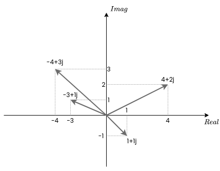
First of all, what is QAM16? To talk about Quadrature Amplitude Modulation, we need first to know what are quadrature signals. In RF, when we want to transmit a signal, we need to split that signal into two different signals with a phase between them of 90 degrees. By doing this, we will have the projection of the signals into two axis. Those axes represent a complex number, being the horizontal axis the real part, and the vertical axis, the imaginary part. Also, we can see those axis using the Euler`sformula, where a signal is split into a cosine signal, that represents the real part, and a sine signal that represents the imaginary part.

\[e^{jx}=cos x + jsin x\]

With this in mind, we will notice that any point can be represented by a complex number. This kind of representation is also known as rectantular. In opposite to the polar form, which represents a point by its module, and its angle.

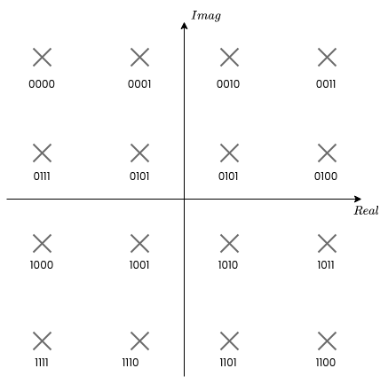
In the XY plane, we have infinite points, so we can encode each of these points with a binary number, and then transmit the value of the real signal and the imaginary signal, the XY coordinates. In practice, we need a separation between each point because the resolution of the DAC used to generate the signal is limited by its number of bits and the SNR. In case of QAM16, we will have 16 discrete points in the XY plane, but the number of points can be increased to QAM32, QAM64, QAM128… The number of points will depend of the features of the device used.

At this point, we know that we need to generate two different signals, the value of those signals will depend on the value we want to transmit, and that value will be sent in packages of 4 bits since each of the points represents a value between 0 and 15. Let’s begin doing some simulations in MATLAB.

First of all, we need to define the binary value that will represent each point in the XY plane. I have chosen these values.

% create symbols dictionary
values = [-3-3j, -1-3j, 3-3j, 1-3j, -3-1j, -1-1j, 3-1j, 1-1j, ...
    -3+3j, -1+3j, 3+3j, 1+3j, -3+1j, -1+1j, 3+1j, 1+1j];

Then I generated a random signal using those values (symbols). Since the rand function generates values from 0 to 1, we need to multiply the value by 15. Then, since list indexes in MATLAB begin with one instead of zero, we also need to add one to the final result. Finally, cast all as an integer to eliminate the fractional part. The value obtained will be the index of the list generated before.

% create symbols
nSymbols = 16;
qamType = 16;

frame = values(int8((qamType-1) * rand(1,nSymbols))+1) 

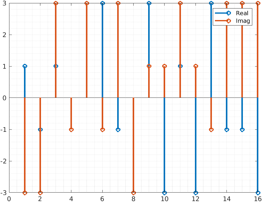
The signal generated will show like the next.

Since the signal is generated from binary data, the signal is discrete and the symbols of the signal are represented by deltas. The harmonic content of all of those delta signals is infinite. That means that the bandwidth needed to transmit the signal without information loss is also infinite, which is in practice impossible. We need to reduce the bandwidth of the signal to be able to transmit and reproduce that signal. To do that we need to make the transition between one symbol and the next softer. We can do that by adding a filter, but the filter will need some samples to perform the transition, so we also need to add some points between each symbol, in other words, we need to upsample the signal.

Upsample a signal in MATLAB is very easy, we only have to use the command upsample.

% apply zero stuffing to upsample the signal
upFactor = 10;

frameUp = upsample(frame,upFactor)

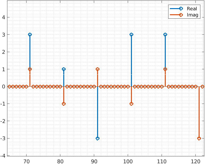
This command will add samples with a value of zero between each sample of the original signal. The number of zero samples will be defined by upFactor.

Now we have to filter the signal to generate the points for interpolating each symbol. To filter the signal, we are going to use a Raised-Cosine filter. This filter is an FIR filter to which we will apply a specific window. The result is a filter that almost eliminates the interference between symbols. We have mentioned that each symbol is a delta, or an impulse. When we compute the DFT of an impulse we will obtain a sinc signal, with an infinite tail. This tail will be added to the next symbols, so its value will be distorted. The tail of the Raised-cosine filter is also infinite but its value is zero when the next symbol is transmitted, so the interference that one symbol produces over the next is almost zero, in other words, the Raised-Cosine filter reduces the inter-symbol interference (ISI). To compute the coefficients for the Raised-Cosine, we will use the rcosdesign command in MATLAB.

% rrc filter
filtlen = 5;
rolloff = 0.25;
b = rcosdesign(rolloff,filtlen,upFactor);

b = b/sum(b); % normalizing coefficients

This function has 3 arguments, the first one is the roll-off, which indicates the excess bandwidth that we will allow to the filter. A small value of this argument will generate softer transitions, and a large value means higher bandwidth, so the transition will be faster. The second argument is the length of the filter, which is the length of the tail of the filter. In my case, I have had good results with a length of four of five. This argument is proportional to the number of taps since they will be the length of the filter (in symbols) multiplied by the upsampling factor. For this case, since the upsampling factor is ten, the order of the filter will be 10 times the length. Now with the coefficients vector obtained from the Raised-Cosine filter, we can filter the signal.

frameUpFiltRe = filter(b,1,real(frameUp));
frameUpFiltIm = filter(b,1,imag(frameUp));

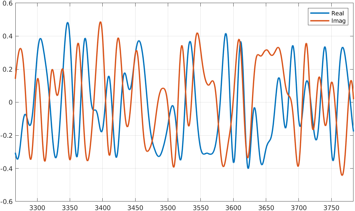
The resulting signals are shown in the next plot.

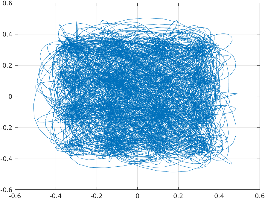
Now, to see exactly the QAM16 modulation, we need to plot both signals again, but using one of them as the X axes.

figure
plot(frameUpFiltRe, frameUpFiltIm);
grid on

And the result is the next.

In the last plot, we see the signal’s entire trip. if we want to see the exact point of the symbol, which in this case is one every ten points, we can use the scatter command with the signal and the upsampling rate.

% scatter plot
txvect = frameUpFiltRe + j*frameUpFiltIm;

scatterplot(txvect, upFactor)

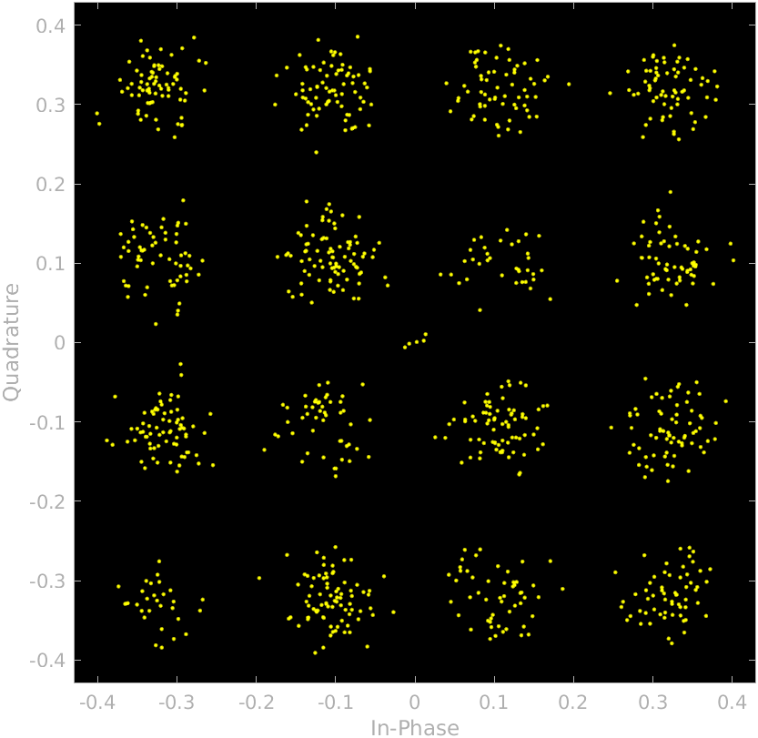
This command will show us the next plot.

We can see how the samples are distributed according to the QAM16 shape. Then, once the signal is transmitted, the receiver will filter again the signal with the same filter, so the dispersion of the points that represent each symbol will be reduced. In this case, we talk about the Root Raised-Cosine filter, since the gain of the transmitter filter will be the root square of the final gain, to keep the gain when both filters are in series.

Now, we are going to move the QAM16 encoder from MATLAB to Verilog. The design is divided into three different blocks.

The first module is qam16_data_packet which will split the input data into 4 bits packages. The output data rate of this module is determined by the next module. Since I have used an AXI4 Stream interface, this module will hold the same output until the next module sets the m_axis_tready signal. Regarding the slave interface, this module will set the s_axis_tready signal when the 8 packages have been sent to the next module.

/* packet counter is increased when receiver is ready to accept data and there is an active 
    transaction (packet_counter > 0), or a new data is received (s_axis_tvalid) */
always @(posedge aclk)
  if (!resetn) begin
    m_axis_tdata <= 4'd0;
    packet_counter <= 3'd0;
    m_axis_tvalid <= 1'b0;
  end
  else 
    if (m_axis_tready && (s_axis_tvalid_reg || (packet_counter > 0))) begin
      m_axis_tdata <= s_axis_tdata_reg[5'd3+{packet_counter, 2'b00} -:4];
      packet_counter <= packet_counter + 1;
      m_axis_tvalid <= 1'b1;
    end
    else
      m_axis_tvalid <= 1'b0;

The next module is named qam16_data_upsampler, and is in charge of the encode the input data into a QAM16 symbol, and also include the zero stuffing samples to upsample the input data. The encoding is made using a kind of dictionary, one for the real part and another for the imaginary part. I have used a modulation_gain signal which is defined as a parameter. With the value of this parameter I can change the amplitude of the output signal. In practice, this gain will act as programmable gain amplifier.

initial begin
  modulation_real_dict[0] <= -16'sd3 * modulation_gain;
  modulation_real_dict[1] <= -16'sd1 * modulation_gain;
  modulation_real_dict[2] <= 16'sd3 * modulation_gain;
  modulation_real_dict[3] <= 16'sd1 * modulation_gain;
  modulation_real_dict[4] <= -16'sd3 * modulation_gain;
  modulation_real_dict[5] <= -16'sd1 * modulation_gain;
  modulation_real_dict[6] <= 16'sd3 * modulation_gain;
  modulation_real_dict[7] <= 16'sd1 * modulation_gain;
  modulation_real_dict[8] <= -16'sd3 * modulation_gain;
  modulation_real_dict[9] <= -16'sd1 * modulation_gain;
  modulation_real_dict[10] <= 16'sd3 * modulation_gain;
  modulation_real_dict[11] <= 16'sd1 * modulation_gain;
  modulation_real_dict[12] <= -16'sd3 * modulation_gain;
  modulation_real_dict[13] <= -16'sd1 * modulation_gain;
  modulation_real_dict[14] <= 16'sd3 * modulation_gain;
  modulation_real_dict[15] <= 16'sd1 * modulation_gain;
end

initial begin
  modulation_imag_dict[0] <= -16'sd3 * modulation_gain;
  modulation_imag_dict[1] <= -16'sd3 * modulation_gain;
  modulation_imag_dict[2] <= -16'sd3 * modulation_gain;
  modulation_imag_dict[3] <= -16'sd3 * modulation_gain;
  modulation_imag_dict[4] <= -16'sd1 * modulation_gain;
  modulation_imag_dict[5] <= -16'sd1 * modulation_gain;
  modulation_imag_dict[6] <= -16'sd1 * modulation_gain;
  modulation_imag_dict[7] <= -16'sd1 * modulation_gain;
  modulation_imag_dict[8] <= 16'sd3 * modulation_gain;
  modulation_imag_dict[9] <= 16'sd3 * modulation_gain;
  modulation_imag_dict[10] <= 16'sd3 * modulation_gain;
  modulation_imag_dict[11] <= 16'sd3 * modulation_gain;
  modulation_imag_dict[12] <= 16'sd1 * modulation_gain;
  modulation_imag_dict[13] <= 16'sd1 * modulation_gain;
  modulation_imag_dict[14] <= 16'sd1 * modulation_gain;
  modulation_imag_dict[15] <= 16'sd1 * modulation_gain;
end

When the symbols are defined, when new data is received at the input, the module checks if the filters are ready to accept new data, if they do, the module sends the first data, and then repeats the same action sending zero data according to the parameter upsampling_factor. Also, a delay between data sending is executed in the state 2'b11- This delay will set the data rate of the system.

case (qam16_upsampler_state)
  2'b00: begin /* waiting for a new input data */
    if (s_axis_tvalid) qam16_upsampler_state <= 2'b01;
    else qam16_upsampler_state <= 2'b00;

    upsampling_counter <= 0;
    m_axis_real_tdata <= 14'd0;
    m_axis_imag_tdata <= 14'd0;
    m_axis_real_tvalid <= 1'b0;
    m_axis_imag_tvalid <= 1'b0;
    prescaler_counter <= 0;
  end
  2'b01: begin /* waiting for receiver ready signal */
    if (m_axis_real_tready && m_axis_imag_tready && (upsampling_counter < upsampling_factor)) qam16_upsampler_state <= 2'b10;
    else if (m_axis_real_tready && m_axis_imag_tready && (upsampling_counter == upsampling_factor)) qam16_upsampler_state <= 2'b00;
    else qam16_upsampler_state <= 2'b01;

    upsampling_counter <= upsampling_counter;
    m_axis_real_tdata <= m_axis_real_tdata;
    m_axis_imag_tdata <= m_axis_imag_tdata;
    m_axis_real_tvalid <= 1'b0;
    m_axis_imag_tvalid <= 1'b0;
    prescaler_counter <= 0;
  end
  2'b10: begin /* write new data. Diration 1 clock cycle */
    qam16_upsampler_state <= 2'b11;

    upsampling_counter <= upsampling_counter + 1;
    m_axis_real_tdata <= (upsampling_counter == 0)? modulation_real_dict[s_axis_tdata]:16'd0;
    m_axis_imag_tdata <= (upsampling_counter == 0)? modulation_imag_dict[s_axis_tdata]:16'd0;
    m_axis_real_tvalid <= 1'b1;
    m_axis_imag_tvalid <= 1'b1;
    prescaler_counter <= 0;
  end
  2'b11: begin /* prescaler for new data and go to wait receiver ready */
    if (prescaler_counter == prescaler_factor) qam16_upsampler_state <= 2'b01;
    else qam16_upsampler_state <= 2'b11;
    m_axis_real_tvalid <= 1'b0;
    m_axis_imag_tvalid <= 1'b0;
    prescaler_counter <= prescaler_counter +1;
  end
endcase

The next modules are the FIR filters for the Raise-Cosine filter. For these filters, I have used the FIR Compiler IP from the Vivado catalog. regarding the coefficints of the filter, I have added to my MATLAB code a small snippet that generates a COE file with the coefficients computed by the rcosdesign command.

% create coe file
nbits = 20;
bq = int32(b*(2^20));

file = fopen( 'rcos_coeff.coe', 'wt' );

fprintf(file, "Radix = 10;\nCoefData= ");

for i = 1:length(bq)
  fprintf(file, ' %f', b(i));

  if (i < length(bq))
    fprintf(file, ',\n');
  else
  fprintf(file, ';');
  end
end
fclose(file);

For the coefficients, I have selected a quantification of 20 bits, which is high enough for this filter.

on the FIR Compiler configuration, we have to select as a source of the coefficients, the file we have created. Making this, we can run the MATLAB script and the FIR Compiler will take the last coefficients automatically.

Then, on the Implementation tab, we have to configure the quantification of the coefficients to 20 bits, as we have configured in the MATLAB script.

Finally, to save FPGA resources, we are going to configure the data rate of the filter. This configuration will not change the response of the filter, and it is not related to the filter itself but is related to the implementation. On the Channel Specification tab, we can configure the input data rate and the filter clock frequency. The DSP Slice spends a clock cycle to compute an operation, so if the number of operations that the DSP Slice must execute, is less than the number of clock cycles between samples, the FIR filter only will use 1 DSP Slice. Making this has a disadvantage. The logic used is increased to implement the needed logic to share the DSP Slice.

Finally, the last module is the driver for the ZMOD DAC.

To generate sample data, I have added a module named qam16_data_generator which generates a 32 bit data when the m_axis_tready signal is set. Once we have implemented all the modules, we can create the block design.

We can see in the block design that I have added an ILA to verify the correct behavior of all the modules. Once the FPGA is configured, the data generator module will run and data will be sent to the DAC and the ILA. If we take a capture using the ILA, using the tcl command write_hw_ila_data, we can export the ILA data to a csv file, and then open it using MATLAB.

write_hw_ila_data -csv_file /home/pablo/workspace/matlab/qam16/ila_data.csv [current_hw_ila_data] -force

Exporting data to MATLAB, and plotting it with two axes, we can see how the QAM16 is generated correctly.

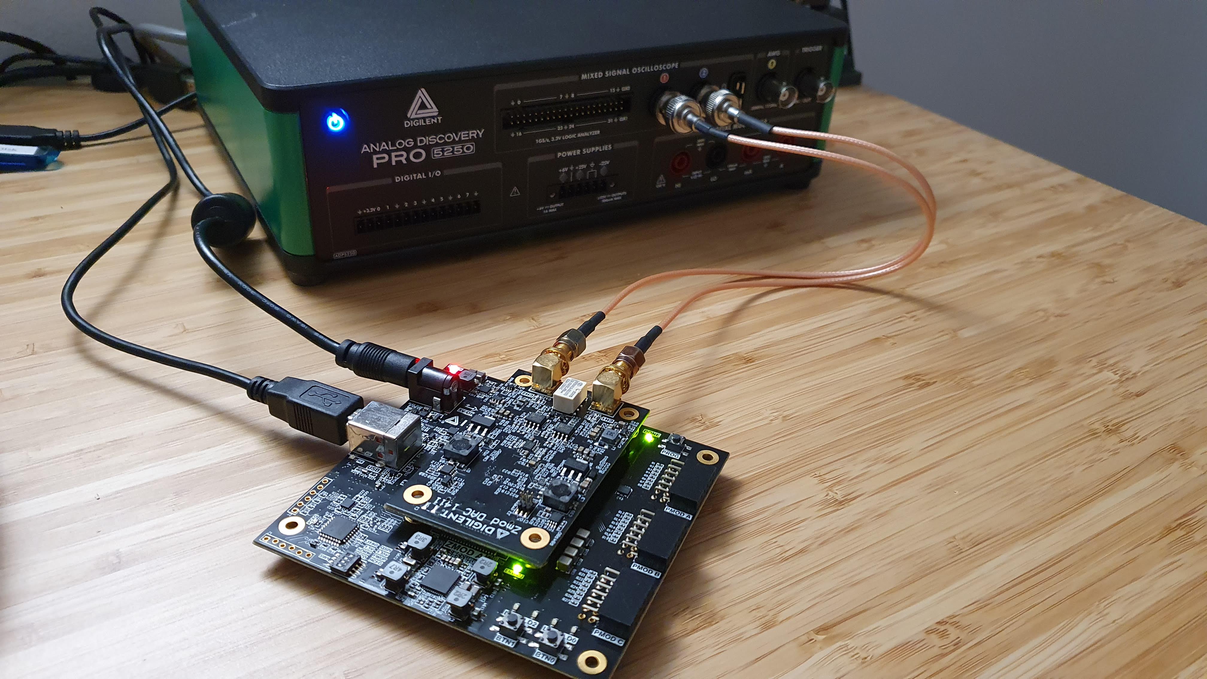
Finally, is time to test the design in the FPGA. I have used the USB104 board, which is based on Artix 7, and also have a SYZYGY socket. To generate the analog signal I have used the ZMOD AWG also from Digilent. Both output channels are connected to the ADP5250.

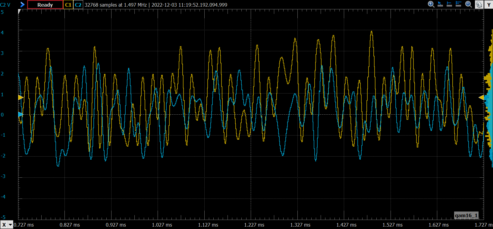
The next capture shows the analog signals captured by the ADP5250.

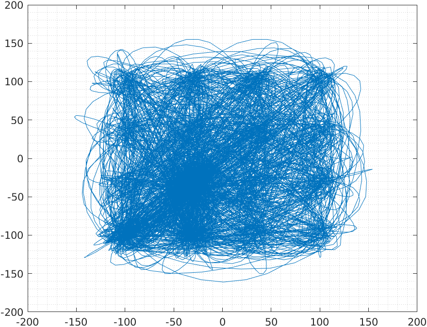
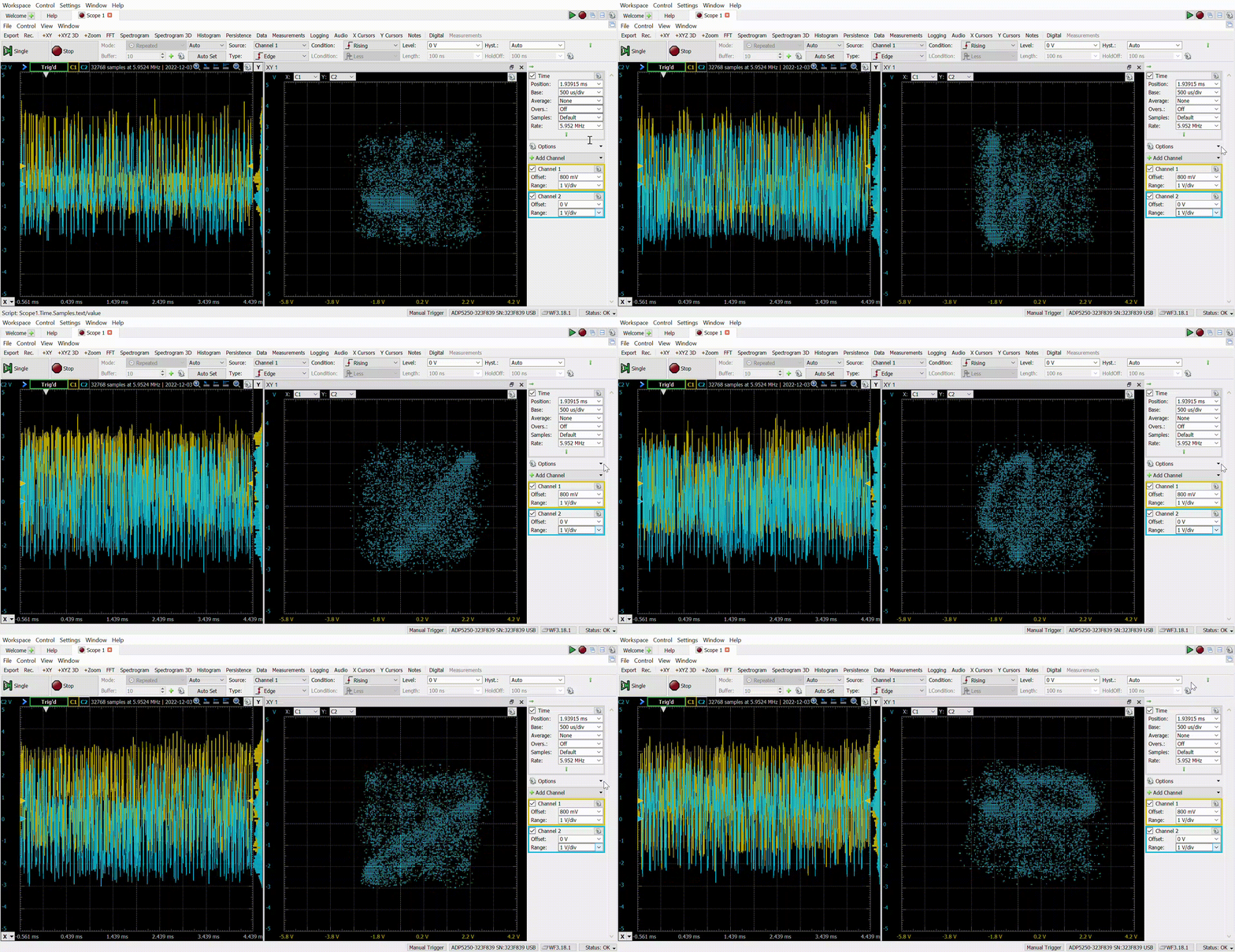
Finally, if we add an XY plot, the result is the next.

The adjustment of the Raised-Cosine filter is not the better, but the result is great! As I mentioned before, I like to develop these kinds of projects because they mix FPGA and digital signal processing for real-world applications. Usually, when we are using GNU Radio or MATLAB to execute this kind of modulation, we do not realize what we are doing exactly, and sometimes we can not achieve good results because of that. Going deep into the implementation of QAM16 or any other modulation, we will understand all the steps needed to make this possible, and this will give us the power to configure the receiver knowing what we are doing. The next step is the receiver, which is a little bit more complicated because we have to add a synchronization algorithm. All the files of this project are available on Github.