Digital control loops. Theoretical approach.
In this blog, I have tried to show you different tools, usually in the field of digital signal processing, so you can select the correct tools for your projects. This time we will use the tools that we have used in other posts but for a different purpose, we are going to design a digital control loop. As the content could be so extensive for a single post, I am going to divide the design in two different posts. In the first one I will talk about digital control loops from the theoretical point of view. Then, in the second one, I will show you how implement and test the algorithm on an FPGA.
Digital control loops are used in many fields of engineering, and for many different purposes. We can find them in the control of switching converters like power supplies, and they are responsible to keep stable the output voltage or current of the power supply, even when a perturbation is introduced in the system like a suddenly change of load. Also digital control loops are very common in communications systems. They are involved in the control of variable gain amplifiers (VGAs), used to keep the input/output power stable, and also in the carrier recovery algorithms, which are responsible of synchronizing the carriers of emitter and the receiver. This last application if the one that we are talking about.
Typical schema of a digital control loop is shown in the next figure. You can find a reference input, used to set the desired output of the system, also we can find a feedback input to read the value of the current output, with the corresponding gain or transfer function (F(z)), used to obtain how close or far is the output from the reference, in other words, the error. That error will be connected to the regulator (R(z)), that will be responsible to keep that error as close as zero as possible. Finally the output of the regulator will be connected to an actuator, that will act over the system (G(z)) in order to modify its output.

Each of the elements of the diagram will have its own transfer function, and we can compute two different loop transfer functions, the open loop transfer function and the close loop transfer function.
\[Gol(z)=R(z)\cdot G(z)\cdot F(z)\] \[Gcl(z)=\frac{R(z)\cdot G(z)}{1+R(z)\cdot G(z)\cdot F(z)}\]Regarding the application we are going to design, we have to consider that when we are designing a communication system, the clock of the transmitter is different than the clock of the receiver. Since the frame sent by the transmitter is synchronized with its own clock, the receiver has to synchronize its clock with the clock received in the frame. Notice that although the clock is different in both devices, the frequency must be the same, however the algorithm we are going to design should be capable to synchronize with the receiver clock even when the frequency of both devices is not exactly the same.
Combining what we already know about the elements of the digital control loops, and the application itself, we will need an element on which the control action will act. That element must generate a clock with a frequency proportional to the output of the regulator, this task will be done by a Numerically Controlled Oscillator (NCO). The algorithm used to obtain the error between the input clock and the generated clock will be a phase detector, and finally we will use a regulator to keep the error closest to zero as possible, that as we will see, we have two different options to use as regulator.
First of all we are going to talk about the phase detector. The purpose of this element is to obtain a signal proportional to the phase error between the wave received and the wave generated by the receiver. There are several types of phase detectors, but most of them are based on mixers (multiplicators), and trigonometric functions. For this projects we are going to use the next relation.
\[sin(\alpha) \cdot cos(\beta)= \frac{sin(\alpha-\beta)}{2}+\frac{sin(\alpha+\beta)}{2}\]If we take a look to our old books about trigonometric, we can see that exists a zone where the relation it is satisfied. If we plot both terms of the equation, and the relation mentioned before, we obtain the next figure.
\[h1 = \frac{sin(\alpha-\beta)}{2}\] \[h2 = \frac{\alpha-\beta}{2}\] \[h3 = \frac{sin(\alpha+\beta)}{2}\]
The code to generate this wave. is the next.
close all
clear all
clc

%% approx
t = -0.01:0.0001:0.01;

f1 = 100;
f2 = 200;

h1 = sin(2*pi*f1*t - 2*pi*f2*t)/2;
h2 = (2*pi*f1*t - 2*pi*f2*t)/2;

h3 = sin(2*pi*f1*t + 2*pi*f2*t)/2;

figure
plot(t,h1);
hold on;
plot(t,h2);
plot(t,h3)
xlim([-0.005, 0.005])
ylim([-1, 1])
legend('h1', 'h2', 'h3')
We can see the two different sine waves, the first of them have a frequency that is the difference between and , and as we have said, the zone closest to zero can be approximated as a proportional term, and the second one is a sine wave with a frequency that is the sum of and . Assuming that the error of the timing recovery algorithm will be less than pi in the major of cases, we can replace the first term for the proportional term. The resulting equation will be the next.
\[sin(\alpha) \cdot cos(\beta)= \frac{sin(\alpha-\beta)}{2}+\frac{sin(\alpha+\beta)}{2}\approx\frac{\alpha-\beta}{2}+\frac{sin(\alpha+\beta)}{2}\]Now we have a term that is proportional to the phase error, and a second term that has a frequency very close to the double of the input frequency, so we can filter that signal and keep only the proportional term.
Once we have the error in phase of the timing recovery algorithm, we have to make that error as closest to zero as possible. The algorithm responsible of doing that, will be the regulator. At this point, we have several options that we can use as regulator, but we will reduce our options to two, the most used. We can use a proportional regulator (P), where the error is used as control action after apply a gain, and the second one is to use a proportional – integral regulator (PI). Lets take a look to the first one.
The schema for the P regulator is as simple as the next figure. It has the advantage that is very simple to implement and we only need to use a multiplicator, which is very efficient if we are thinking in the FPGA implementation.

On the other side, the P regulator has a disadvantage, but before we need to talk about the type of the systems. The type of the systems is related to the number of integrators of the system, that are poles in the origin in continuous systems. If the system has no poles in the origin, we say that the system is a type 0 system, on the other hand, if the system has one pole in the origin, the system will be a type 1 system, also if it has two poles in the origin, the system will be a type 2. Each type has different responses. lets start with type 0. A type 0 system could be the next.
\[H(s)=\frac{1}{(s+2)(s+3)}\]We can see a system that has 2 poles, but no one in the origin. Lets see its step response and its ramp response.

G0 = 1/((s+2)*(s+3));
Gcl0 = feedback(G0,1);

figure
sgtitle('Type 0 System')
subplot(1,2,1)
step(Gcl0)
subplot(1,2,2)
step(Gcl0/s, 100)
title('Ramp response')
hold on
step(1/s)
We can see that the response of the system when a unit step is applied do not reach the unit value. Moving this to our application, we can say that the phase error will never reach zero. Also I have obtained the ramp response. This plot shows the system response when a ramp is applied to the input. In the application we are designing, the ramp response is very important because a difference in frequency between the input and the output is translated in a ramp of phase error. In this case we can see how the ramp response diverge from the reference, so the system will never be able to follow a difference in frequency.
The solution could be add an integrator and convert the type 0 system to a type 1 system. In this case, the transfer function I am going to use is this.
\[H(s)=\frac{(s+1)(s+3)}{s(s+2)(s+3)}\]The plots obtained for this system are the next.

We can see for the type 1 system that the unit step response reaches the unit value, so we will not have phase error in steady state. For the ramp response, we can see that the response is better, since unlike the type 0 system, where the ramp error increases with time, for the type 1 system the ramp error is constant. For our application this translates into perfect frequency tracking, but with a constant phase error.
Can we do it better? of course! we can use a type 2 system below.
\[H(s)=\frac{(s+1)(s+3)}{s^ {2}(s+2)(s+3)}\]The plots for this system are the next.

Finally, for this kind of systems we can see how both the step response and the ramp response reach the input value. For the timing recovery algorithm we will use a type 2 system since we need that the receiver clock will be synchronized both in phase and frequency.
Once we know the type of system we need, we have to obtain the schema or the transfer function of the regulator. The proportional term have been shown above, now we need to obtain the integral term. In a continuous system we already see that add an integrator to the system is simply multiply by . At this point, to use the integrator in a digital system we need to discretize the integrator using any of the discretization methods that exist. One of the discretization methods is the Impulse Invariance. This method is based in separate the transfer function in a series of first order systems. To do that we can apply the partial fraction decomposition. Then, for each term, we have to apply the next replacement:
\[\frac{1}{s-a}=\frac{T}{1-e^{aT}z^ {-1}}\]If we apply this substitution to the integrator equation, since \(a=0\), the resulting equation is the next.
\[H(z)=\frac{T}{1-z^ {-1}}\]Impulse invariance is not the only method we can use. Other easy to apply method that we can use is the bilinear transformation. This method use the next substitution.
\[s=\frac{2}{T} \cdot \frac{1-z^ {-1}}{1+z^ {-1}}\]Applying this transformation to the integrator continuous equation, we will obtain a new discrete transfer function.
\[\frac{1}{s}=\frac{T}{2} \cdot \frac{1+z^ {-1}}{1-z^ {-1}}\]The difference between these two methods is the position of the zero in the map. For the impulse invariance method the zero is located in the origin, on the other side, using the bilinear transformation locate the zero in -1,0.

Comparing the response of two transfer function we will see that the increasing ratio is the same, but for the impulse invariance method the steps start in ts, however for the bilinear method the first sample has a ts/2 level.

If we combine the proportional action, given by a gain, and the integral action, we can will obtain the best of both types of regulators. For the step response, the proportional action will improve the fast response of the regulator, and then, once the error is reduced, the integral action will reach the reference.
In the figure below you can find the three options of regulator to control the output of the system.

At this point you can see that the regulators that I have explained only have one integrator, so they are a type 1 system. Before I have said that we will have to use a type 2 system in order to make 0 the frequency error, and you are completely right, but also me. When we are working with systems that involves regulators, we have to consider the integrators of the entire close loop transfer function. For this system, the low pass filter has no poles in the origin, so is a type 0 system, the regulator has one integrator, therefore now, we have a type 1 system, and finally, the missing integrator is located in the NCO, and I am going to explain that.
The NCO is an element which output is a sine wave which frequency is proportional to its input. If I keep constant the input, the output of the NCO will be a sine wave of a constant frequency, but what about the phase? The phase increases in a rate that is proportional to the input, and this is an integrator, the second that we need to have a type 2 system. The model of the NCO is the next.
\[H(z)=K\cdot \frac{T}{1-z^ {-1}}=[rad]\]Notice that the output of the NCO are radians, not radians/sec.
Now is time to verify if all that I have said until now is true. To verify the algorithm I have used a Simulink model that has as input an NCO with a fixed frequency of \(fs/2+200\) . To that frequency I have added a step of 200 at 0.15s. The integrator starts in \(\pi\), that is translated in a phase shift of \(\pi\) radians. As a phase detector, I have used a multiplicator followed by a second order butterworth filter, that is calculated in the workspace. Then I have added a PI regulator, with the constants declared in the workspace, and I have used the impulse invariance method to discretize the integrator. Finally we have a complex NCO. The sine output has to be the same as the input signal, and the cosine output is used as feedback for the phase detector.

First of all, we will test the system configuring the ki to 0. That will produce a type 1 system, since the only integrator in the system is in the output NCO. The low-pass filter is configured at 600 Hz in order to obtain only the DC level. Since the fs is 100 ksps, the input NCO frequency will be 20 kHz + 200 Hz which I have added as frequency error. The filter has to attenuate the twice of that frequency, 40.4 kHz. Notice that I have added an adder that sums the configured frequency of the receiver, that is fs/5. This feedforward will help the regulator, and it works like the tunning frequency of the receiver.
% pi regulator
ki = 0;
kp = 2000;

% filter
fc = 600;
wn = 2*fc/fs;
[b,a] = butter(2,wn);
With this configuration, when the systems starts, the regulator have to fix the frequency error and also de phase error. We can see in the upper plot the output of the filter, the error, and in the bottom plot the input and the output sine waves. We can see how the type 1 system (ki = 0), how the algorithm is able to follow the frequency, but it can’t reach a phase error of zero. We have a constant error in the phase since the phase error, due to the difference in frequency, is a ramp.

After apply the step at 0.15s, again we can see the same result, a constant error in phase.

The next is configure the ki of the regulator to a value different than zero.
% pi regulator
ki = 400000/fs;
kp = 3000;

% filter
fc = 600;
wn = 2*fc/fs;
[b,a] = butter(2,wn);
Now we can see how when the simulation starts, the phase error is zero after 5ms, and both input and output sine waves are synchronized.

After the step, the systems takes 20ms to keep its output stable and the output NCO synchronized.

The speed of this system is limited by the filter we are using in the phase detector. Is easy to understand that the regulator can not be faster than the filter, since the regulator will increase, or decrease its output and the filter response will not respond until a time after. To improve the speed of the system, I have changed the cut-off frequency of the filter to 1000 kHz. This will make that the attenuation of the filter will be lower, but we will see a significantly improvement in the speed.
% pi regulator
ki = 600000/fs;
kp = 6000;

% filter
fc = 1000;
wn = 2*fc/fs;
[b,a] = butter(2,wn);
With this configuration we can see how the system is synchronized in less than 3ms.

But the biggest improvement of the system is the response to the step.

With this configuration we can see how the phase error is reduced to the half, which is almost unnoticeable in the sine waves.
The configuration that I have used is far to be the best, but is very funny test different configurations to check how the response of the system changes, and also how modifying the configuration of the filter makes the system to accept higher Kp or Ki configurations. The next step is implement this system in an FPGA and verify its behavior.
All the files are available in Github.