Downsampling using MATLAB and the Microchip's Icicle kit.
 Icicle kit
Many times we need to manage low-frequency signals sampled at high rates. This can be due to the need to detect edges in that signal as fast as possible, for example, if we are using that signal to protect a device. This kind of situation makes the filters used to obtain a clean low band have to be high-order filters due to the ratio between the sampling frequency and the cut-off frequency. In this situation, resampling the signal at a lower rate can help us with the design of the filter. In this post, I will show you how you can perform a downsampling of a signal without distortion. IN addition, we are going to implement that algorithm in a Microship’s PolarFire SoC.
I have created a signal that contains several harmonics and also a main tone at 50Hz, which is the signal of interest. The ADC I have used has a sampling frequency of 100 Ksps. The signal acquired is shown in the next figure.

As I mentioned before, the example signal has a DC component, generated by a PWM signal, and the signal of interest is a sine of 50Hz. The signal has also several harmonics above 2 kHz, and the harmonics generated by the square signal at multiples of the square signal frequency. The frequency spectrum of the signal is the next.

If we make zoom between DC and 2KHz, we can see that only 2 components are present in that range, the DC and the main harmonic of the signal, a 50Hz tone.

The signal I have generated is very common when we are reading the AC grid voltage or current, and we have connected to that grid several switching converters with different switching frequencies. In many cases we will need to measure the RMS of the 50 Hz component. To compute a true RMS, we need to store several cycles of 50Hz. For a 100 ksps signal, the number of samples to store five cycles is 10 000 samples.
\[n_{samples}=\frac{100e3}{50} \cdot 5 = 10000\]Since we do not need that number of samples, we can downsample the signal, that is to take one sample every \(n\) samples. For example, if we apply a downsampling factor of 32, (making it a power of two will make easiest the HDL code), we will use to compute the RMS only one sample every 32 samples, so the resulting number of samples will be 312. That’s great!
The resulting sampling frequency can be obtained with the next equation.
\[f'_{sample}=\frac{f_{sample}}{DF}=\frac{100e3}{32}=3125 Hz\]Being \(DF\) the downsampling factor.
If we apply that decimation factor to the signal, the resulting waveform is the next.

Oh wait, if we pay attention to the signal, seems like the 50hz waveform, which we can see clearly in the 100 ksps signal, is deformed. Also, the signal has high-frequency harmonics, which can be normal since the original waveform also has them. To check what exactly happened, let’s calculate the FFT of the signal.

In the frequency spectrum of the signal, we can see how in the range between DC and the new Nyquist Frequency, 1562 Hz, have appeared different tones that are not in the original signal. To explain it, we can take a look at the next figure.

The first frequency spectrum shows the tones when the sampling frequency are the original one, 100 ksps. In that case, all the components of the signal, the bandwidth of the signal, is located below half of the sampling frequency, below the original Nyquist frequency, so the acquisition is made correctly, and there is no aliasing. The second spectrum shows the result when we decimate the samples, obtaining a new sampling frequency. The tones of the signal are the same, but this time, there are several components above the new Nyquist frequency, so these components or images appear in the first Nyquist zone, distorting the signal with components even below the fundamental tone at 50Hz.
At this point, to avoid the aliasing effect when we are going to apply a decimation, we need the first filter to attenuate the most as possible all the components that will remain above the new Nyquist frequency. Also, to avoid distortion in the filtered signal, we will need a symmetrical FIR filter. The solution seems easy, let’s calculate an approximation of the order of the filter. We can do that using the next equation.
\[N=\frac{Atten}{22(\frac{f_{stop}}{f_{sample}} - \frac{f_{pass}}{f_{sample}})}\]The new sampling frequency will be 3125 so we need to attenuate all the components above 1562 Hz. As the original signal has no components between 50 Hz and 2000 Hz, we can set the f stop in 2000, and the f pass must keep the amplitude of the 50hz component, so we can configure the pass frequency at 500Hz. The attenuation at 2000 Hz will be set at 40 dB. Using the above equation, the order calculated is 121. To compute the FIR filter with these parameters, I have used the next MATLAB code.
% filter compute (one stage decimator)
atten = 40; % attenuation required in dB
fstop = 2000;
fpass = 500;
n = atten / (22*(fstop/fsample - fpass/fsample));
taps = fir1(floor(n),fpass/fsample);
Now, to test the filter + decimator circuit, I have designed in Simulink the next diagram.

The FFT of the resulting signal is, as expected, a clean frequency spectrum with no aliasing.

Now we have performed a one-stage decimation. The elevated order of the filter is due to the ratio between the sampling frequency and the bandwidth that is of interest to us, in this case, DC to 500Hz. If when we will implement this algorithm in an FPGA, the elevated order of the filter could be a problem or not. For example, if we use the Microship’s Icicle kit, it is based on the PolarFire SoC MPFS250T, which has 784 multipliers (18×18), the number of multipliers is not a big issue but the effort of Libero to connect 122 multipliers could generate congestion problems in the FPGA. Also, consuming 15% of the multipliers in only one filter is not a great idea.
The solution for that is to use folding. MATLAB can implement FIR filter. In case we want to use only one multiplier, we can configure the architecture of the FIR block as Fully Serial, so all the multiplications will be performed by only one multiplier. On the other hand, the clock of the filter must be 122 times faster than the clock enable.

The intermediate solution would be the better choice. We can select the number of multiplication branches we want, therefore each multiplicator will perform a 122/n multiplications, and the clock frequency is reduced to 122/n times faster. To do that, we need to configure the architecture as Partly Serial and configure the Serial partition as [25 25 25 25 22], which means that we will use 5 multiplicators, and four of them will perform 25 multiplications and the fifth will perform 22, that makes a total of 122, and we need a clock “only” 25 times faster than the clock enable.

Even with that, we have a 122 order FIR filter, which is a large FIR filter. Would be great if we can reduce the order of the FIR filter while keeping the behavior of the decimator, and this is exactly what we can achieve using a two-stage decimator. Two-stage decimator uses 2 sets of FIR + Decimator. The structure is the next.

The total downsampling factor will be M1*M2, and the total multiplications for the FIR filters will be n+p+2. The key of this method is to select the appropriate values for M1 and M2 that makes n and p lowest as possible. In the paper write by L. Crochiere and L.Rabiner, they expose an equation to calculate the optimum value of M1.
\[M1_{OPT} \approx 2 \cdot M \cdot \frac{1-\sqrt{\frac{MF}{2-F}}}{2-F(M++1)}\] \[F=\frac{f_{stop}-B'}{f_{stop}}\]The value of \(B’\) is the bandwidth that we want to retain, in our case this frequency will be 500, as we configured before. And the \(F_{stop}\) will be the same as used before, 2000 Hz. With these values, the approximate M1 optimum value is 9, so the M2 value will be the integer near the result of 32/9 which is 4. These values will produce a total downsampling factor of 36. For this example, this is valid because our goal is to reduce the number of samples to store for a true rms compute. If you need an exact value of M, you must select M1 near the optimum that makes M1*M2 the exact factor you need.
With this configuration of M1 and M2, we have at the end of the first stage a sampling frequency of 11 111 Hz (100e3/9), and at the end of the second stage, we have a sampling frequency of 2777 Hz.
To design the first FIR filter, we will configure the pass frequency as our pass frequency of interest, that is 500 Hz, the same used above. And the stop frequency can be configured in any value between \(f_{pass}\) and 11 111 / 2. To achieve the minimum order for this filter we will configure the fstop as the Nyquist frequency, that is 5 555 Hz. Using an attenuation of 40 dB, the estimated order of the FIR filter is 35. We will repeat the steps to compute the estimated order for the second FIR filter, using as \(F_{pass}\) 500 Hz, and \(F_{stop}\) the Nyquist frequency for the second stage, that is 2777 / 2 = 1388 Hz. With this configuration, the order of the second FIR filter is 22. The MATLAB code to do that is the next.
% Filter compute (two stage decimator)
signal_bw = 500;
f = (fstop-signal_bw)/fstop;
m1_th = floor(2*dowsampling_factor*(1-sqrt(dowsampling_factor*f/(2-f)))/(2-f*(dowsampling_factor + 1)));
m2_th = floor(dowsampling_factor / m1_th) + 1;
m1 = m1_th;
m2 = m2_th;
% m1 = 16;
% m2 = 2;

fstop1 = fsample/m1/2;
fpass1 = 500;

n1 = atten / (22*(fstop1/fsample - fpass1/fsample));

taps1 = fir1(floor(n1),fpass1/fsample);

fsample2 = fsample/m1;
fstop2 = fsample2/m2/2;
fpass2 = 500;

n2 = atten / (22*(fstop2/fsample2 - fpass2/fsample2));

taps2 = fir1(floor(n2),fpass2/fsample2);
The Simulink schema to test this configuration is shown below.

Executing this model, and calculating the FFT of the output, we will obtain the next result for the first stage.

We can see how the band between DC and 2000 Hz is kept clean, so there is no aliasing in our signal. Since the \(f_{stop}\) is configured at 5555 Hz, we can see some components in the band below 5555 Hz, which is expected.
The output of the second stage is shown below.

We can see that the only component that remains in the baseband is the 50Hz tone and the DC component as expected. This spectrum is similar to the one achieved with the 122 th order filter. This time, we have used 2 FIR filters of 35 th order and 22 th order, so the total number of multiplications is 35 + 22 + 2 = 59. We have divided the total number of multiplications by a factor of 2. The resulting signal is that you can see below.

Now we have to implement this in the PolarFire SoC of the Icicle Kit. To generate the IP, we will modify the diagram to create a subsystem only with the two-stage downsampler.

Now we must set the precision in the convert block. In my case, I will use an ADC of 12 bits, so I will configure a fixed-point format signed, 12 bits of width and 11 bits for the decimal part.

Now inside the subsystem, we have to configure the precision of the coefficients and the internal registers of the FIR filters. The configuration will be the same for both filters.
For the coefficients, we must take into account that the multipliers of the PolarFire SoC have a width of 18×18 bits, so if we select a width greater than this, the Libero will use 2 or more multiplicators per multiplication. In this case, the coefficients do have not very small values, so a precision of 16 bits, with 15 bits for the decimal part will be enough. The input width is configured before from the convert block, and for the product output and accumulator widths, we will let MATLAB choose them. The configuration of the FIR filters will be the next.

When we configure the corresponding data types, when we execute the model, Simulink returns a warning indicating that a precision loss has occurred. This is normal since we are translating a floating-point value of 32 bits to a fixed-point value of 16 bits. This will change the behavior of the filters since the coefficient values have changed. The deviation to the floating-point coefficients could be analyzed by plotting the bode diagram of the filter with the original and the quantized coefficients or adding all the coefficients to compute the gain of the filter. Since the width of 16 bits is far enough, both bode diagrams seem the same, so I have added the coefficients to compute the gain.
% compute quantize coefficients

nt = numerictype(true,16,15); % define the width of the quantization

taps_fi = fi(taps);
taps_q = quantize(taps_fi,nt);

gain_fir_q = sum(taps_q)

taps1_fi = fi(taps1);
taps1_q = quantize(taps1_fi,nt);

gain_fir1_q = sum(taps1_q)
gain_fir1_q = sum(taps1)
We can see that the gain is kept almost the same, having an error of the 0.05 %.
Now we are going to open the HDL coder properties by right click on the subsystem. On the first window, we can configure the language, which is configured to Verilog for me, and the name of the output folder. Next in the target tab, we can select the device we are using. Since PolarFire SoC is not available in the R2021b release, we can select a similar device like the PolarFire FPGA, and a target frequency of 50MHz.

Finally, in the Report tab, we will enable all the Optimization Reports. Regarding the implementation of the FIR filters, the easy way is to keep the same clock frequency for both filters, so the folding factor must be the same. In this case, we will use a folding factor of 4, so the configuration for the first FIR filter, which has an order of 35 will be [4 4 4 4 4 4 4 4 4] using 9 multipliers, and for the second FIR filter which has an order of 22, the configuration will be [4 4 4 4 4 3].

Finally, we can generate the HDL for Subsystem. When the HDL is generated, we can see the reports. If we open the High-Level Resource Report, we can see that the number of multipliers is 15, nine for the first filter and six for the second one.

If we take a look at the code, we can see that the decimators are implemented in the file named two_stage_downsampler_tc, and its content can be a bit complicated. First of all, you need to know that the external clock_enable signal must be four times faster than the data input rate. This is due to that FIR filters use four clock_enable cycles to compute each output (folding factor of four). Now, we can see that the module generates six different clock_enable signals.
// enb_4_1_1 : identical to clk_enable
// enb : 4x slower than clk with last phase
// enb_4_9_1 : 9x slower than clk with phase 1
// enb_1_9_0 : 36x slower than clk with last phase
// enb_1_9_1 : 36x slower than clk with phase 1
// enb_1_36_1 : 144x slower than clk with phase 1
The first one is connected to the first FIR filter, and it is the same signal as the input clock_enable, remember, four times faster than the data rate. Then, the signal enb is four times slower, so this will be the rate of the output data of the first FIR filter. The next signal is nine times slower than the original clock enable, and this signal will be connected to the clock enable of the second FIR filter, since nine is the downsamplig factor of the first stage. Then two signals 36 times slower are generated. These signals are connected to the register that join both filters, and 36 is the result of 4 times multiplied by the downsamplig factor of the first stage. In our case, the input clock enable has a rate of 4×100 ksps, the output of the first FIR filter is four times slower due to the folding factor, so we divide 4×100 ksps by four, then the downsampling rate of the first stage is nine, so we divide by nine, in the end, 4×100 ksps/36. Finally, a last clock enable is generated 144 times slower, that is the result of multiplying the last clock enable by the downsampling factor of the second stage, 4x9x4 = 144, and this will be the output clock enable. The output rate can be calculated as 4×100 ksps/144 = 100 ksps/36 which is the output rate designed.
Also, on the top level generated we can see some register to equilibrate the delays of the different modules.
Now, we have the IP core generated, so the next is open Libero and instantiate the two_stage_downsampler module.
Once we have Libero opened, we must create a new project for the PolarFire Device.

Then we will add all the files created by MATLAB, and also a top file created to instantiate the two-level downsampler, the ADC driver, the clock generators and a clock enable generator.

Now we will instantiate the oscillator. PolarFire SoC devices have two internal oscillators, one running at 2 MHz, and the other one at 160 MHz. In this case, 2 MHz is too slow so we will use the 160 MHz oscillator.

Since 160 MHz is a high frequency, we will connect to the output of the oscillator a Clock Conditioning Circuit (CCC) to reduce the rate of that clock.

Now we must instantiate the CCC from the catalog tab.

To configure the CCC we must set the input frequency to 160 MHz, and the output frequency to 40 MHz. Also, we need to enable the PLL Lock output to use it for the Reset circuit.

Once we have these two components in our design, we must instantiate them in the top level. To verify the behavior of the algorithm we will output the signal through a PWM modulator. Also, we need to include a clock enable with an output 100 slower than the 40 MHz clock, that is a 400 kHz.

Once we have all the components instantiated, we will synthesize the design. Then we must create the constraints file. In the reference design of the icicle Kit, we can find several pdc files with the different output ports of the board. One of those files has the configuration for the Raspberry Pi connector, that is the connector we will use to connect the ADC and the PWM signal. The content of the constraints file is shown below.
set_iobank -bank_name Bank1  \
    -vcci 3.30               \
    -fixed true             \
    -update_iostd true

set_io -port_name pwm_output -pin_name C9 -fixed true -DIRECTION OUTPUT -io_std LVCMOS33

set_io -port_name spi_miso \
    -pin_name G12    \
    -fixed true    \
    -io_std LVCMOS33  \
    -DIRECTION INPUT

set_io -port_name spi_sclk    \
    -pin_name C10    \
    -fixed true    \
    -io_std LVCMOS33  \
    -DIRECTION OUTPUT

set_io -port_name spi_mosi    \
    -pin_name D13    \
    -fixed true    \
    -io_std LVCMOS33  \
    -DIRECTION OUTPUT

set_io -port_name spi_ss    \
    -pin_name H13    \
    -fixed true    \
    -io_std LVCMOS33  \
    -DIRECTION OUTPUT
With this file modified, we can implement the design and also program the board. When the design is implemented and the board is programmed, the PWM output will start switching. The PWM module has clocked from the 160 MHz clock, so we will obtain a switching frequency of 160e6/4096 = 39 KHz, so we can filter the signal with a first-order RC filter.
To test the algorithm, I have used a 50 Hz signal, to verify that the input and the output of the signal are the same but delayed.

Then I have used a 10 kHz signal that is attenuated for the two stage downsampler.

Is very common in many fields to use analog to digital converters with rates hundreds of times faster than the signal we need to acquire. The reasons are 2, first, the cost of a 500 ksps ADC is low, so for the same price we chose the faster one. Second, even if the signal we need to acquire was a low-frequency signal, in some cases we need to see fast changes in this signal to detect an edge, for example, if we need to protect the system with this measure. In those cases, we can downsample the signal that we will use to measure and keep the high rate to the signal we will use to protect. In these cases, downsampling is the solution, but we need to know what happened when we downsample the signal, because of that, we need to know the signal. In this post, I have tried to show you how I will proceed in these cases, and applications like MATLAB can help us to make the design faster. Also, if we join MATLAB with the power of a big FPGA like the PolarFire SoC, with more than 700 multiplicators, we can do almost any algorithm.