[AN001] Designing from zero an IIR filter in Verilog using biquad structure and bilinear discretization.
Filtering is likely the most common DSP algorithm that any embedded engineer has to design, no matter it they are developing for an STM32, or TI DSP or, of course, en FPGA. Filtering is such important because the majority of the applications are connected to the real world, so they need to capture real signals with the undesirable elements that all real signals have, i.e noise, offset… Also, signals that we need to acquire, not always will be the dominant signals we acquire, for example, for biological signals, we will acquire a high level of 50 or 60 Hz corresponding with the grid frequency. On this cases we will need a filter.
As you sure know as reader of this blog, on digital systems, we have 2 kind of filters, FIR (Finite Impulse Response) filter, which only use the value of the input now and the value on the past, and IIR (Infinite Impulse Response), which use the value of the input now and in the past, and also the value of the past outputs. FIR filters are easy to design for many applications, but them response are limited for a low order filters. On the other hand, with IIR filters, we can achieve more aggressive responses, but they have the disadvantage that the filter can be unstable in certain cases. On this article we will see how we can implement a second order filter step by step, from the filter design up to it verilog implementation.
The process to design an IIR filter is always the same. First of all we have to design the filter using its continuous transfer function, then, once the natural frequency of the filter, the order and the quality factor are selected, we will obtain the corresponding \(s\) function. The next step in order to digitalize that filter, is apply some transformations to replace the variable \(s\) by \(z\), this process is known as discretization. In order to discretize the continuos transfer function we can use several methods, and one of the easy to use methods is Tustin, or the bilinear transform.
The bilinear transform is based on replace the \(s\) variable in the continuous transfer function by a function of \(z\). In the next example we can see discretize a single pole low pass filter applying the bilinear transformation. The replacement we have to perform in the continuos transfer function is the next.
\[s=\frac{2}{ts}\left(\frac{1-z^{-1}}{1+z^{-1}}\right)\]For a single pole filter, these will be steps to perform the bilinear transform. The equation of a low pass single pole filter is the next:
\[h(s) = \frac{1}{1+\frac{s}{\omega_N}}\]Applying the transformation, we have:
\[h(z) = \frac{1}{1+\frac{2}{ts} \cdot \frac{1-z^{-1}}{1+z^{-1}} \cdot \frac{1}{\omega_N}}\]operating with the denominator to obtain a common denominator,
\[h(z) = \frac{ts \cdot (1+z^{-1}) \cdot \omega_N}{ts \cdot (1+z^{-1}+2(1-z^{-1})}\]then, we need to separate the elements with \(z\), of the others, and finally we will have a \(z\) function that depends of the sampling frequency and the natural frequency of the filter.
\[h(z)=\frac{ts\cdot \omega_N + ts\cdot \omega_N z^{-1}}{ts\cdot \omega_N+2+(ts\cdot \omega_N-2)z^{-1}}\]In MATLAB, we can do this transformation using the command hz = c2d(hs,ts,'Tustin')
The entire MATLAB code for a 100 hz low pass filter is the next.
%% single pole filter discretization

% continuos filter declaration
s = tf('s');

% define characteristics of the filter
fc = 100;

% compute angular frequency
wc = 2*pi*fc;

% Write the transfer function of a low pass single pole filter
hs = 1/(1+s/wc);

% show its bode diagram
bode(hs)

% discretization using tustin method

fs = 100e3;

ts = 1/fs;

hz = c2d(hs,ts,'Tustin')
The result for hz is
hz =

  0.003132 z + 0.003132
  ---------------------
       z - 0.9937

Sample time: 1e-05 seconds
Discrete-time transfer function.
In order to verify that the equation we have obtained manually is correct, we have to create a transfer function using the values we have obtained before.
hz_man = tf([ts*wc, ts*wc],[ts*wc+2 ts*wc-2], ts)
the result in this case is
hz_man =

  0.006283 z + 0.006283
  ---------------------
     2.006 z - 1.994

Sample time: 1e-05 seconds
Discrete-time transfer function.
We can see that, dividing numerator and denominator by 2.006, the equation is the same as the one obtained usint the c2c command.
The bilinear transform, line any other discretization method, is an approximation, so we will introduce some errors. The size of that errors are related to the sampling frequency since a very (very very) high sampling frequency, in some cases, could seem continuous. In real systems, where the sampling frequency depends of the ADC and many real components, we can use high sampling frequences, but in other cases we will introduce a significantly error.
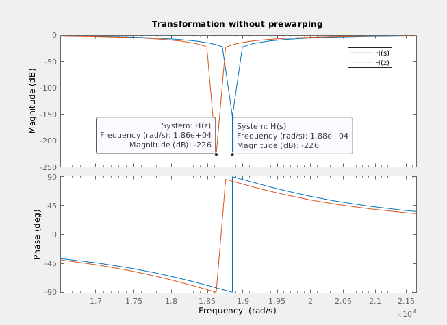
In case of the bilinear transform, one of the errors that we will introduce is the frequency warping. This effect produces a shift of the natural frequency of the filter. This effect may be negligible in the case of a low pass filter, but in case of narrow band filters, the error could make that the filter don’t work.
In order to find the error caused by the bilinear transformation, we need to find the relation between the analog frequency and the discrete frequency . First of all, we will start with the equation of the bilinear transformation.
\[s=\frac{2}{ts}\left(\frac{1-z^{-1}}{1+z^{-1}}\right)\]Replacing \(z\) by its polar form \(e^{j \omega d}\), we have
\[s=\frac{2}{ts}\left (\frac{1-e^{-j \omega d}}{1+e^{-j \omega d}}\right)\]Now, we are going to split the exponential using the half-angle.
\[1-e^{-j \omega d} = e^{-j \omega d/2} (e^{j \omega d/2}-e^{-j \omega d/2}) = e^{-j \omega d/2} \cdot 2j sin(\omega d/2)\] \[1+e^{-j \omega d} = e^{-j \omega d/2} (e^{j \omega d/2}+e^{-j \omega d/2}) = e^{-j \omega d/2} \cdot 2 cos(\omega d/2)\]Replacing in the above equation for the numerator and the denominator, we have:
\[s=\frac{2}{ts}\left ( \frac{e^{-j \omega d/2} \cdot 2j sin(\omega d/2)}{e^{-j \omega d/2} \cdot 2 cos(\omega d/2)}\right) = \frac{2j}{ts}\cdot tan(\omega d /2)\]Now, we are going to split the exponential using the half-angle.
\[1-e^{-j \omega d} = e^{-j \omega d/2} (e^{j \omega d/2}-e^{-j \omega d/2}) = e^{-j \omega d/2} \cdot 2j sin(\omega d/2)\] \[1+e^{-j \omega d} = e^{-j \omega d/2} (e^{j \omega d/2}+e^{-j \omega d/2}) = e^{-j \omega d/2} \cdot 2 cos(\omega d/2)\]Replacing in the above equation for the numerator and the denominator, we have:
\[s=\frac{2}{ts}\left ( \frac{e^{-j \omega d/2} \cdot 2j sin(\omega d/2)}{e^{-j \omega d/2} \cdot 2 cos(\omega d/2)}\right) = \frac{2j}{ts}\cdot tan(\omega d /2)\]Then, we have to find the relation with the analog , so we are going to equal both equations
\[\sigma + \omega a j = \frac{2j}{ts}\cdot tan(\omega d /2)\]We can verify that the real part is 0, and the imaginary part, witch $\omega a$ is directly
\[\omega a = \frac{2}{ts}\cdot tan(\omega d /2)\]Notice that the limit when \(t_S\) tends to zero, is \(\omega a = \omega d\).
In MATLAB, we can check this deviation easily. In this case we will declare a second order continuous band-stop filter. And then discretize the filter using the Tustin method.
close all
clear all
clc

% define filter
fc = 3000;
wn = 2*pi*fc;
q = 5;%1/sqrt(2); % butterworth

s = tf('s');

h = (s^2+wn^2)/(s^2+wn/q*s+wn^2)

%bode(h)

% discretize filter
fs = 100e6/2048 % prescale FPGA frequency by factor of 2048
ts = 1/fs;

hz = c2d(h,ts,'tustin');
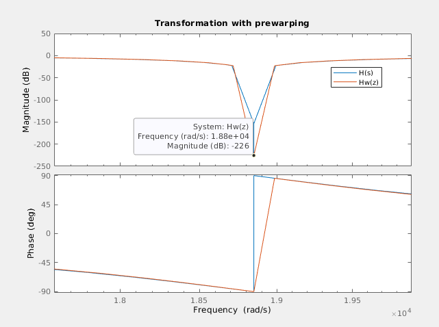
We can see how the frequency of the digital filter is moved. Then we will apply the pre-warping to the natural frequency, and re discretize the filter using this new frequency.
% calculate prewarping
wp = 2/ts*tan(wc*ts/2);
hw = (s^2+wp^2)/(s^2+wp/q*s+wp^2)
hwz = c2d(hw,ts,'tustin');
We can se how in this case, both frequencies are the same, so the error is fixed.
In order to verify this behavior in the real world, we are going to implement this second order band stop filter in Verilog, and then we will check the warping error, and then how using pre-warping we can fix it.
Before start coding, we have to think what we want of the module we will create. In my case, is very important be able to parametrize the module, this way, in case I change the width of the input, or the width of the output, that only represents a change on a parameter, without modify the code of the module since it means new tests for the module. Also, we have to think what numeric format we will use. For this kind of filters, is obvious that we will need a signed format, and the capability to manage decimal numbers. To achieve this requirements, we have to select between fixed point and floating point, and for me the decision is clear, I want a code that can be instantiated alone, without an external floating point unit, so the format will be fixed point. If we add the requirement of parameters, and the fixed point format, we will need parameters to define the width of the signals, and also the width of the decimal part, which will be related to the precision we need. Also, the precision, will be selected to obtain a response of the implemented filter as similar as possible to the designed. Now, how many width we need to parametrize? We can define one width that will be used as for inputs and outputs and for coefficients, but this way, the width of the coefficients will be select according the width of the data generator, and for some filters, which the coefficients are on the stability limit, this could represent a problem. So, at least we will define 2 different widths, one for the input and outputs, according the data drain and the data source, and other one according the resolution we will need. Another thing we have to think about widths, are the resolution of the internal operations, because in some cases, an stability problem is not related to the width of the coefficient itself, but the operation resolution, so at this point, will be interesting decoupling the width of the coefficients that will be generated on MATLAB or Python, with the width of the internal filter operations. Finally, filter parameters will looks like the next.
parameter inout_width = 16,
parameter inout_decimal_width = 15,
parameter coefficient_width = 16,
parameter coefficient_decimal_width = 15,
parameter internal_width = 16,
parameter internal_decimal_width = 15
Next we have to think on the interfaces. Applications where data is transferred between modules in a continuous way, AXI4-Stream will be the best option. On the inputs and output field, we will define both master and slave AXI4-Stream interfaces to acquire and send data. Although the input and output widths are parametrize, if we want to connect the module to an existing AXI4-Stream IP, this width are restricted to the width of the bus.
input aclk,
input resetn,

/* slave axis interface */
input [inout_width-1:0] s_axis_tdata,
input s_axis_tlast,
input s_axis_tvalid,
output s_axis_tready,

/* master axis interface */
output reg [inout_width-1:0] m_axis_tdata,
output reg m_axis_tlast,
output reg m_axis_tvalid,
input m_axis_tready,
Regarding the coefficients, the best to insert them is with an AXI4-Lite interface, but I want to design this module without the need of use a Zynq or Microblaze, so the easy way to insert the coefficients are as inputs.
/* coefficients */
input signed [pw_coefficient_width-1:0] b0,
input signed [pw_coefficient_width-1:0] b1,
input signed [pw_coefficient_width-1:0] b2,
input signed [pw_coefficient_width-1:0] a1,
input signed [pw_coefficient_width-1:0] a2
Now, with all the inputs and outputs defined, we have to think on the data flow. First, as we have different formats defined, to be able to perform operation between the coefficients and data, we have to change the format of all signals to the internal format, which is defined by the internal width and the decimal width. The integer width used is defined as a localparam, and is corresponding with the difference between the width and the decimal width. To change the format, we will fill with zeros the low side of the signal until the decimal part will be completed. For the integer part, as the format used is signed, we have to perform a sign extension, that is fill with the value of the MSb until the integer part will be completed. Notice that this works because the internal width are bigger or equal to the inout and coefficients width.
/* resize signals to internal width */
assign input_int = { {(internal_integer_width-inout_integer_width){s_axis_tdata[inout_width-1]}},
                          s_axis_tdata,
                          {(internal_decimal_width-inout_decimal_width){1'b0}} };
assign b0_int = { {(internal_integer_width-coefficient_integer_width){b0[coefficient_width-1]}},
                          b0,
                          {(internal_decimal_width-coefficient_decimal_width){1'b0}} };
assign b1_int = { {(internal_integer_width-coefficient_integer_width){b1[coefficient_width-1]}},
                          b1,
                          {(internal_decimal_width-coefficient_decimal_width){1'b0}} };
assign b2_int = { {(internal_integer_width-coefficient_integer_width){b2[coefficient_width-1]}},
                          b2,
                          {(internal_decimal_width-coefficient_decimal_width){1'b0}} };
assign a1_int = { {(internal_integer_width-coefficient_integer_width){a1[coefficient_width-1]}},
                          a1,
                          {(internal_decimal_width-coefficient_decimal_width){1'b0}} };
assign a2_int = { {(internal_integer_width-coefficient_integer_width){a2[coefficient_width-1]}},
                          a2,
                          {(internal_decimal_width-coefficient_decimal_width){1'b0}} };
Digital filter, both FIR and IIR, need to store the value of the past inputs, and IIR also the value of the past outputs, so we will need a pipeline structure to store the past values.
/* pipeline registers */
always @(posedge aclk)
  if (!resetn) begin
    input_pipe1 <= 0;
    input_pipe2 <= 0;
    output_pipe1 <= 0;
    output_pipe2 <= 0;
  end
  else
    if (s_axis_tvalid) begin
      input_pipe1 <= input_int;
      input_pipe2 <= input_pipe1;
      output_pipe1 <= output_int;
      output_pipe2 <= output_pipe1;
    end
Now, the next is perform the filter calculations. a second order filter need to perform 5 multiplications, and remember that it does not necessary mean that the modules uses 5 DSP slices. The code I developed performs combinational multiplications. This allows 0 clock cycles delay, but limit the speed of the filter. If your timing constrains are not met, you can register the input of the multipliers, and then make a retiming to let Vivado select where is more efficient put the register.
/* combinational multiplications */
assign input_b0 = input_int * b0_int;
assign input_b1 = input_pipe1 * b1_int;
assign input_b2 = input_pipe2 * b2_int;
assign output_a1 = output_pipe1 * a1_int;
assign output_a2 = output_pipe2 * a2_int;
The result of the multiplications will be added, in case of the input, and subtracted in the case of the outputs, to obtain the filter output. As the output of the product has a size of twice of the operands, the addition must be the same width. To use the output on the multiplications, we have to perform a shift to delete extra decimal positions. Regarding the extra integer position will be truncated on the assignment.
assign output_2int = input_b0 + input_b1 + input_b2 - output_a1 - output_a2;
assign output_int = output_2int >>> (internal_decimal_width);
Finally, the value of the output will be reformatted to the inout widths.
assign m_axis_tdata = output_int >>> (internal_decimal_width-inout_decimal_width);
Regarding the AXI4-Stream management signals, as the filter behaves as bridge, with one cycle delay, management signals will pass through the filter with one cycle delay.
At this point, we have the Verilog module implemented and ready to be used as band-stop filter. The next is obtain the coefficients in MATLAB using the tfdata function. Regarding the width of the filter, we are going to use 18 bits of resolution for the decimal part, and 2 for the integer part, in order to let the filter reach up to +-2. The MATLAB code to obtain the coefficients in fixed point is the next.
% filter implemetation

[num, den] = tfdata(hwz)

b0 = num{1}(1)
b1 = num{1}(2)
b2 = num{1}(3)
a1 = den{1}(2)
a2 = den{1}(3)

% quantize

fracBits = 18;

b0_qq = floor(b0*2^fracBits)
b1_qq = floor(b1*2^fracBits)
b2_qq = floor(b2*2^fracBits)

a1_qq = floor(a1*2^fracBits)
a2_qq = floor(a2*2^fracBits)
This return the next result.
b0_qq =

      252631


b1_qq =

     -468081


b2_qq =

      252631


a1_qq =

     -468081


a2_qq =

      243119
Once we have the five coeffients, we have to introduce them as inputs in the coefficients inputs in the Verilog module.
  axis_biquad_v1_0 #(
  .inout_width(15),
  .inout_decimal_width(13),
  .coefficient_width(20),
  .coefficient_decimal_width(18),
  .internal_width(20),
  .internal_decimal_width(18)
  ) axis_biquad_inst0 (
  .aclk(clk100mhz),
  .resetn(pll_locked),
  /* slave axis interface */
  .s_axis_tdata({axis_data_signal_ch1[13], axis_data_signal_ch1}),
  .s_axis_tlast(),
  .s_axis_tvalid(&filter_prescaler),
  .s_axis_tready(),
  /* master axis interface */
  .m_axis_tdata(axis_data_signal_filt),
  .m_axis_tlast(),
  .m_axis_tvalid(),
  .m_axis_tready(),
  /* coefficients */
  .b0(20'd252631),
  .b1(-20'd468081),
  .b2(20'd252631),
  .a1(-20'd468081),
  .a2(20'd243119)
  );
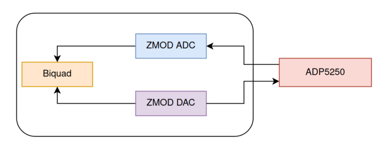
In order to verify that this effect occurs, and it is fixed using pre-warping, I am going to use the Digilent’s Eclypse Z7 with the ZMOD Scope and the ZMOD AWG. Also, to generate the signal and verify the response of the filter I am going to use the brand new Analog Discovery PRO 5250, witch has a signal 125 Msps signal generator as well as a two channels scope capable to acquire up to 1 Gsps.
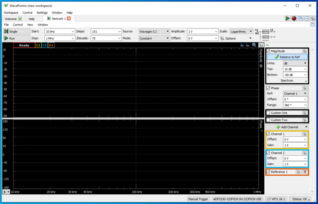
To obtain the natural discretized frequency (\(\omega d\)), I am going to use a very useful function of the ADP 5250, which performs a frequency sweep obtaining for each frequency the gain of the filter, so the result will be the bode diagram of the filter. To configure this mode, we need to open the tool Network.
Once this tool is opened, we need to configure the number of points, and the minimum and maximum frequency. Also we need to configure the amplitude of the signal that the generator will generate. In this case, the natural frequency of my filter is 3 kHz, so the configuration I will use if 1V of amplitude, and a frequency range from 500 Hz to 10 kHz. The number of points will configure the frequency step. In my case, I have changed the number of points according to my needs.
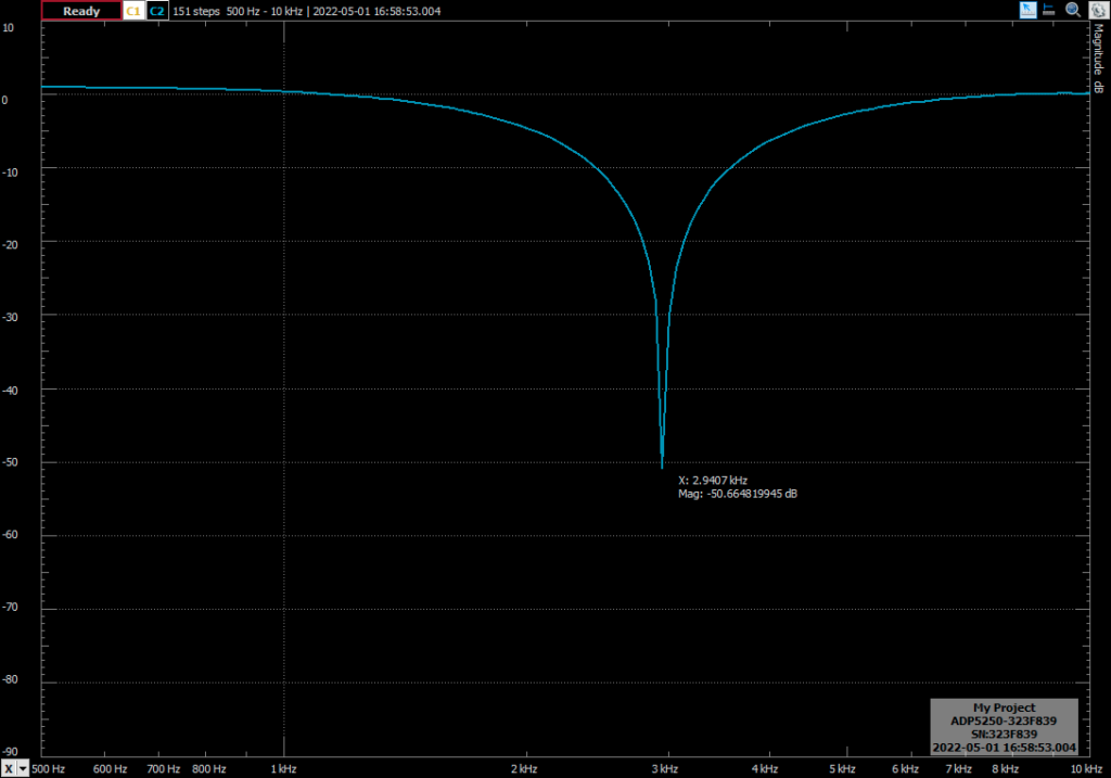
First, I have configured the biquad filter as a band-stop butterworth filter, with a natural frequency of 3 kHz. This time I have not correct the frequency warp. Then, clicking on Single, the ADC 5250 will execute one entire swap. The result is shown in the next figure.
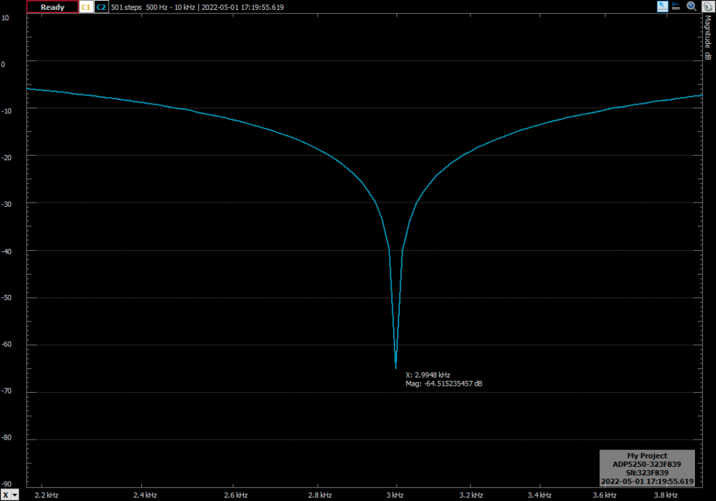
You can see how the response of the filter is the expected, but the natural frequency is 2.9407 khz, which is 59.3 Hz below the expected frequency. Applying the pre-warping to the frequency, the response of the filter is the next (notice that the zoom of the image is different).
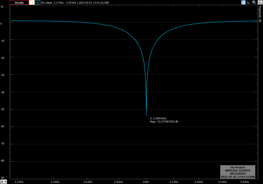
With the frequency correction, the error if 0.0052 Hz, which is a despicable error. In the next test I have increased the quality factor of the filter to 5. This will have effect in the bandwidth of the notch, obtaining a narrower band filter.
The bilinear transformation is widely used to design IIR filters because its simplicity. We only have to replace s in the continuous transfer function by the z function. Other methods like impulse invariance needs of the partial fraction expansion algebra, so the process is a bit more complicated. Also, the bilinear transformation maps the entire s-plane, so there is no aliasing errors. On the other side, it produces a warping in the frequency, but using pre-warping, as we have seen in this post, we can fix that frequency deviation.


