BLDC motor control with the KD240
 KD240
KD240
In the last article, I generated a base project for the KD240 kit from AMD. This kit is based on the Kria K24 SOM, the smallest brother of the K26 SOMs used in the KR260 and KV260. Since this board was released I have been interested in it because, I am not 100% sure of this, it was the first board released by AMD intended to a power electronics system. In this case, the system is a three-phase inverter to control a BLDC motor. It is nice to see that today, in 2024, is not all about AI, although almost all the examples and the articles provided by AMD go in that direction.
The board is very complete, and allows us to read all the variables of the power stage, input DC voltage and current, output AC voltage and current. Having all the variables available allows us to design different kinds of control, for example, a missing variable in most kits like this is the output voltages, which is needed to design a sensorless control, but the KD240 kit has them. All the variables, mixed with all the interfaces that the KD240 give us infinite possibilities. In this article I an going to create the basic modules to make a BLDC motor rotate using this kit. All the modules will be designed in RTL, so we will have the APU and the RPU available for, for example, to perform a high-level control or manage communications.
Three phase systems
First of all, we need to know how BLDC motors work. This kind of motor, unlike regular DC motors, needs a three-phase system. The shape of the voltage waveform applied on each phase depends on the type of control we are going to apply. We can work with two different types of signal, Space-Vector PWM (SVPWM), and Sinusoidal PWM (SPWM). The SVPWM, in summarizing it a lot, uses tables that relate the state of the switches with the spin angle of the rotor. The SVPWM control is more complex that I have explained, so if you want to learn more about SVPWM you can find more information here or here. In this article, I am going to use the second control method, the SPWM. This method consists of generating three sine wave signals with a phase of 0, 240 and 120 degrees. Then, these three signals are used in a PWM modulator in order to generate a PWM signal, and this PWM is applied to the power stage. A motor has two different variables that we can control, the speed of the rotor, and the torque. For BLDC motors, the torque is controlled with the voltage applied to the motor and the speed is controlled with the frequency of the three sine signals applied.
Unfortunately, the fact that the torque and the speed can be controlled with different control actions, they are coupled. The BLDC motors are bidirectional systems, which means that if we apply a voltage to their terminals, the motor rotates, and also, if we rotate the motor, a voltage is generated in their terminals. The value of the voltage is a parameter defined by the manufacturer, and can be found in the motor features as a value followed by “KV”. For example, a value of 1000KV means that the motor generates 1 volt per 1000 revolutions per minute (rpm), and here is where speed and voltage applied are related, if we need to accelerate the motor to 4000 rpm, and keep a constant torque at that speed, we need to apply at least 4 volts to the motor, and then the corresponding voltage to reach que desired torque. Also, since the speed is related to the frequency applied, we need to measure the speed, and apply the frequency that is corresponded with the speed of the motor. In the acceleration process, we will need to increase the voltage, in order to create the torque and produce an acceleration, and at the same time, increase the frequency while the speed of the motor is increased. If this relation is not accomplished, the rotor speed and the electrical frequency will lose synchronism, and the motor rotation will turn irregular.
To generate the three-phase system, we are going to use the vector control theory. We start with a 2 dimensions system where we are going to define a vector. The projections of the initial position of this vector in the real (D) and imaginary (Q) axes are the variables we are going to control. The angle of that vector is \(\phi\). When the vector starts to rotate, the projections of the vector in both axes while the vector is rotating describe two sinusoidal signals delayed \(\pi/2\). We can also see this from the DSP point of view, we have a DC signal which has real and imaginary parts. To start to rotate this vector, we need to multiply by \(e^{j\omega t}\), and the initial vector will increase its frequency to \(\omega t\). The result of this operation is again a real and imaginary vector, that rotates at \(\omega t\), formed by two sinusoidal signals with a delay between them of \(\pi/2\).The equation used in this case is
\[V_{alpha} = V_D cos(\theta)-V_Q sin(\theta)\] \[V_{beta} = V_Q cos(\theta)+V_D sin(\theta)\]This transformation of a pair of static vectors to two rotating vectors in quadrature is named Park inverse transformation, or dq to alpha/beta. Notice that the Park transformation performs the transformation between two quadrature vectors into two static vectors. This is really well explained in this note from Microchip.

At this point, we have two signals delayed \(\pi /2\), but we need a three-phase system. The next step is to decompose the rotating vector into three different vectors delayed 120 degrees that are equivalent to the initial vector. To perform this transformation we are going to use the Clarke inverse transformation or alpha/beta to abc. Again, the Clarke transformation performs the transformation in the opposite direction. The equation is the next:
\[Va = V_{alpha}\] \[Vb = \frac{-V_{alpha}}{2}+\frac{\sqrt{3}V_{beta}}{2}\] \[Vc = \frac{-V_{alpha}}{2}-\frac{\sqrt{3}V_{beta}}{2}\]
Finally, when we have the three sine signals, we can modulate them using Pulse-Width Modulation (PWM). To do that, we have to compare the signals with a triangular carrier signal. The amplitude of the carrier signal is 1, so when a sine signal is above the amplitude of the carrier, the result of the modulation process will be a continuous ‘1’, and the system is overmodulating.

What I have explained here, is a very little part of the theory behind the vector control, but is enough to understand the modules I have designed to control the BLDC motor.
RTL Vector control implementation
In order to generate the correct PWM pattern, I have designed 4 different modules. The first one is the angle_gen.v. This module generates the sine and cosine signals needed to perform the rotation of the initial angle. The cosine and sine signals are stored in a block RAM initialized with the values. The depth of the memory is 4096 points.
reg signed [sincos_width-1:0] sine_signal [(2**angle_width)-1:0];
reg signed [sincos_width-1:0] cosine_signal [(2**angle_width)-1:];

initial $readmemh("../memory_content/sin.mem", sine_signal);
initial $readmemh("../memory_content/cos.mem", cosine_signal);
Then, the address to read will be the angle, which is a 12-bit value, and is increased according to a clock prescaler, so will be using this prescaler how we are going to set the frequency.
\[F{\theta}=\frac{F_{CLK}}{4096 \cdot Prescaler}\]
Now we have the most important block of the system dq2abc.v. This block integrates the Park inverse and the Clarke inverse transformations. In this case, the modulator cannot overmodulate, so I used a fixed point format of 16 bits Q15. The first step is to perform the DQ to alpha/beta transformation.
/**********************************************************************************
*
* DQ to alpha/beta
*
**********************************************************************************/

assign d_cos_2width = d_vector * cos;
assign d_sin_2width = d_vector * sin;
assign q_cos_2width = q_vector * cos;
assign q_sin_2width = q_vector *sin;

assign d_cos = $signed(d_cos_2width >>> inout_decimal_width);
assign d_sin = $signed(d_sin_2width >>> inout_decimal_width);
assign q_cos = $signed(q_cos_2width >>> inout_decimal_width);
assign q_sin = $signed(q_sin_2width >>> inout_decimal_widt);

assign alpha = d_cos - q_sin;
assign beta = q_cos + d_sin;
The output of this module will be two sinusoidal signals, at \(\omega t\) frequency, delayed \(\pi/2\). If the value of Q is zero, alpha corresponds directly with the cosine and beta is the sine.

Now we have the second transformation, which converts from alpha/beta to a three-phase system. For the gain \(\frac{\sqrt{3}}{2}\) I have used a parameter that is auto-calculated according to the fixed point format selected. The rest are just arithmetical operations.
/**********************************************************************************
*
* alpha/beta to abc
*
**********************************************************************************/
assign beta_sqrt3_2_2width = beta * sqrt3_2;

assign beta_sqrt3_2 = $signed(beta_sqrt3_2_2width >>> inout_decimal_width);

assign a = alpha;
assign b = -$signed(alpha>>>1) + beta_sqrt3_2;
assign c = -$signed(alpha>>>1) - beta_sqrt3_2;
The result is now a three-phase system.

The next module is needed because of the way I have used to create the carrier signals. Since I want the PWM frequency will be configurable, I needed a way to change the carrier frequency. To do this we have two methods, a fixed period, which means that the initial and the last value of the carrier are always the same, and the slope is the variable that is modified to modify the frequency. This method has a disadvantage. Since we have a limited resolution, given by the clock frequency, the resolution in the slope are always integer divisors of the clock frequency. This is not a problem with high clock frequencies, and low PWM frequencies, but in some cases, the step between two following divisors could be too big.
To avoid this, I have used the second method, the constant slope. With this method, the carrier slope is always defined by the clock, in other words, the counter used to generate the triangular signal counts every clock cycle, and the frequency of the triangular wave is defined by changing the maximum and the minimum values. This way, the resulting period have a resolution of \(\frac{1}{F_{CLK}}\) seconds.

The disadvantage of this method is that, as I said before, the amplitude of the carrier is 1, so the equivalent 1 for the modulators changes with the PWM frequency, and is here where this module takes importance. This module applies a gain in the modulator to keep the 1 in the carrier period, for example, if I have a modulator of 0.5, that is 16384 in Q15 format, and my carrier has a period of 1000, the operation that this module performs is
\[MOD_{G} = \frac{16384 \cdot 1000}{2^{15}} = 500\]500 is the 0.5 value of the carrier.
/**********************************************************************************
*
* Multiplication by the pwm period
*
**********************************************************************************/
assign mod_a_gained_2width = mod_a * pwm_period;
assign mod_b_gained_2width = mod_b * pwm_period;
assign mod_c_gained_2width = mod_c * pwm_period;

assign mod_a_gained = $signed(mod_a_gained_2width >>> inout_decimal_width);
assign mod_b_gained = $signed(mod_b_gained_2width >>> inout_decimal_width);
assign mod_c_gained = $signed(mod_c_gained_2width >>> inout_decimal_width);
Finally, the modulators with the gain applied are used to generate the PWM signal in the modulator module.
/**********************************************************************************
*
* Carrier generation
*
**********************************************************************************/
always @(posedge aclk)
	if (!resetn)
		up <= 1'b1;
	else
		if (up && (carrier >= pwm_period))
			up <= 1'b0;
		else if (!up && (carrier <= -pwm_period))
			up <= 1'b1;
		else
			up <= up;

always @(posedge aclk)
	if (!resetn)
		carrier <= 0;
	else
		carrier <= up? carrier + 1: carrier - 1;
/**********************************************************************************
*
* Phase comparators
*
**********************************************************************************/
/* phase a comparator */
always @(posedge aclk)
	if (!resetn)
		pwm_a <= 1'b0;
	else
		pwm_a <= ($signed(mod_a > carrier))? 1'b1: 1'b0;

/* phase b comparator */
always @(posedge aclk)
	if (!resetn)
		pwm_b <= 1'b0;
	else
		pwm_b <= ($signed(mod_b > carrier))? 1'b1: 1'b0;

/* phase c comparator */
always @(posedge aclk)
	if (!resetn)
		pwm_c <= 1'b0;
	else
		pwm_c <= ($signed(mod_c > carrier))? 1'b1: 1'b0;
The resulting PWM signals are these.

To test this design I have created a project for the KD240 kit, and generated this block design. The clock of the system comes from one ethernet phy, so we don’t need the PS to generate the clock. Notice that the angle generated does not come from the real speed of the rotor, so in this design, even the motor will rotate, if we try to stop the rotor since there is no torque control or position feedback, it will be desynchronized.

To set the D vector value, PWM frequency and output frequency I have used a Virtual Input/Output module so I can modify the values from the JTAG.

To test this design, you have to adjust the voltage at the output and the output frequency manually to keep the motor rotating. These are the most basic modules needed to make the motor turn, the next will be to use the position sensors of the motor to close the speed loop and keep the rotor synchronized with the stator voltage. The setup I used for this article is this. I have not used the Kria LD240 Accessory Pack because I just need a BLDC motor and a power supply, and I already had them. In addition, the cost of a BLDC motor is just 20 €, and AMD kit is 200 €. if you are interested, the motor I used is the JK42BLS01 from Aliexpress. yes, the AMD’s kit came with a power supply, well, I have used my Lab power supply which costs me 70€.

For a future article, we will check the hall sensor signals of the motor and close the speed and torque loops. All the files of this project are available on GitHub, as well as the scripts needed to create the Vivado project and test the modules.