Designing IIR filters in Python.
Calculating the coefficients of an IIR filter is something familiar in this blog. In general, when I have to design a new filter, I usually do it in MATLAB because I already have a set of scripts to design different types of filters. Things get complicated when, for example, I don’t have a MATLAB available on the computer I am working on, or simply the system I am using is not able to run MATLAB properly, for example, an embedded computer. In these cases, I use Python with two different libraries, Scipy and Control systems. These two libraries allow me to design almost any kind of DSP algorithm at no cost, and with a very low resource usage, so it could run in any embedded computer or SBC. Let’s see how we can use these two libraries.
The first we have to do in a Python script is import the different libraries that we are going to use. In this case, we will use Scipy, for all the DSP algorithms, Numpy for general math operations and Matplotlib for plotting signals.
from scipy import signal
import numpy as np
import matplotlib.pyplot as plt
The algorithm we are going to implement is an IIR filter, which is almost the most generic algorithm we will use. To implement an IIR filter we have several options. In this article, we are going to see two different methods using the Scipy library, and the other one using the Control systems library.
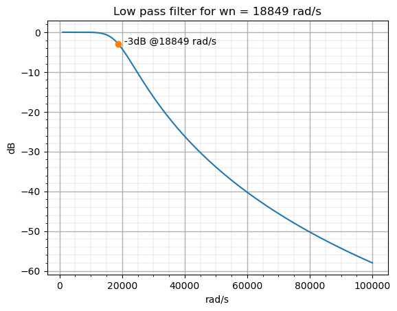
In the Scipy library we have a function named iirfilter, which returns the designed filter coefficients. The use of this function is quite easy for a simple filter, and it can be increasing its complexity when we need to configure whuile we need more customization. The basic arguments of the iirfilter function are the filter order, and the natural frequency of the filter. Also we can define the filter type, the filter response, whether the filter is digital or analog… In the next example, I designed a continuous (analog='true') low-pass filter, with a Butterworth response. For an analog filter, the natural frequency of the filter is defined in radians per second.
## Design a continous iir filter using scipy

N = 4 # filter order
wn = 2*np.pi*3000 # natural frequency in rad/s

# compute the filter coefficients
b,a = signal.iirfilter(N, wn, btype='lowpass', ftype='butter', analog='true')

# calculate frequency diagram
w, h = signal.freqs(b,a)

# plot frequency diagram
plt.plot(w, 20 * np.log10(abs(h)))

# drawing a point on wn,-3dB
plt.plot(wn,-3, 'o')

# text on the point created
plt.text(wn,-3,f'  -3dB @{int(wn)} rad/s', horizontalalignment='left')

# plot title
plt.title(f'Low pass filter for wn = {int(wn)} rad/s')
plt.xlabel("rad/s")
plt.ylabel("dB")

# plot grid
plt.grid(which = "major", linewidth = 1)
plt.grid(which = "minor", linewidth = 0.2)
plt.minorticks_on()
Besides the design of the filter, in the script we can see also the plotting of the response, and also a point in the coordinates \(\omega_n\), -3dB, which is where the natural frequency of a Butterworth filter is.
Obviously, with the function iirfilter we can also design a digital filter. To do this, we have just to remove the argument analog='true'. In addition, the way in which the natural frequency is given to the function changes. In this case, the \(\omega_n\) is given in a number between 0 and 1, being 1 the equivalent to \(\pi rad/sample\). In this case, I declared a new variable named fNyq which has the value of the sampling frequency divided by two. Then we have just to divide the natural frequency of the filter by the Nyquist frequency, and the resulting value will be in a range of 0 to 1, being one the half of the sampling frequency.
# Design a discrete iir filter using scipy

N = 4 # filter order
wn = 3000/fNyq # natural frequency between 0 and 1

# compute the filter coefficients
b,a = signal.iirfilter(N, wn, btype='lowpass', ftype='butter')

# calculate frequency diagram
w, h = signal.freqz(b,a)

# plot frequency diagram
plt.plot(w/np.pi, 20 * np.log10(abs(h)))

# drawing a point on wn,-3dB
plt.plot(wn,-3, 'o')

# text on the point created
plt.text(wn,-3,f'  -3dB @{wn} pi', horizontalalignment='left')

#plot title
plt.title(f'Low pass filter for wn = {wn} pi')
plt.xlabel("pi rad/sample")
plt.ylabel("dB")

# plot grid
plt.grid(which = "major", linewidth = 1)
plt.grid(which = "minor", linewidth = 0.2)
plt.minorticks_on()
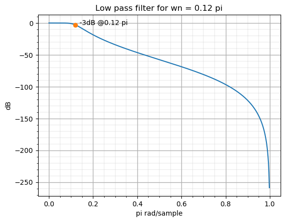
The resulting frequency response is the next. I have changed the labels on the figure to be consistent with the new way of obtaining the natural frequency.
The iirfilter also gives us the choice if give it the sampling frequency, and then we can give it the natural frequency in the same units as the sampling frequency given. The idea is that the division is made inside the function. The next example makes this.
# Design a discrete iir giving sampling frequency filter using scipy

N = 4 # filter order
wn = 3000 # natural in same unit as fs

# compute the filter coefficients
b,a = signal.iirfilter(N, wn, btype='lowpass', ftype='butter', fs=fSample)

# calculate frequency diagram
w, h = signal.freqz(b,a)

# plot frequency diagram
plt.plot(w/np.pi, 20 * np.log10(abs(h)))

# drawing a point on wn,-3dB
plt.plot(wn/fNyq,-3, 'o')

# text on the point created
plt.text(wn/fNyq,-3,f'  -3dB @{wn/fNyq} pi', horizontalalignment='left')

#plot title
plt.title(f'Low pass filter for wn = {wn/fNyq} pi')
plt.xlabel("pi rad/sample")
plt.ylabel("dB")

# plot grid
plt.grid(which = "major", linewidth = 1)
plt.grid(which = "minor", linewidth = 0.2)
plt.minorticks_on()
The response of the system is exactly the same as before since the filter has not changed, just the way of computing the natural frequency has changed.
The filter we designed in the above examples is a fourth-order filter, so the number of coefficients that the function has returned is five for the numerator and five for the denominator, as long as they are different than zero. In reality, when we are going to implement a filter in an FPGA or a DSP, we will tend to implement a series of first and second-order filters in series. This is done because the coefficients will be greater than the ones used for high-order filters, so the quantification error will be increased, or even will make that filter, which is stable in the design, turns unstable due to small errors in quantification. This is more important when we have a resonant filter, with poles near the unity circle. In this case, we need to take the coefficients for the fourth-order filter, and obtain an equivalent set of two second-order filters, that, connected in series, have the same response as the fourth-order filter. This set of second-order filters is known as second order sections. In the scipy library we can obtain the second order sections of a high-order filter using the function tf2sos, but using the function iirfilter, we can obtain directly the filter as an array of second-order filters coefficients. To do this, we need to pass to the function the argument output='sos'.
sos = signal.iirfilter(N, wn, btype='lowpass', ftype='butter', output='sos')
The variable sos has the value of 2 sets of 6 coefficients, which are the needed for a second order filter (three for the numerator and three for the denominator).
Coefficients:
[[ 0.00482434  0.00964869  0.00482434  1.         -1.04859958  0.29614036]
 [ 1.          2.          1.          1.         -1.32091343  0.63273879]]
For those that use to work in MATLAB, the commands of the Scipy library are quite unfamiliar. If we need, or just want to feel more comfortable, using MATLAB like commands, there is another Python library that can help us, the control system.
To import this library to our script, we just to add the next line.
import control as ct
Now, if we need to design a completely customizable filter, with non-standard response, we will need to implement and test a custom transfer function, for example like the next.
\[h(s)=\frac{\frac{\omega_n}{Q}s}{s^2+\frac{\omega_n}{Q}s+\omega_n ^2}\]This cannot be done with the iirfilter function, but with this library we can generate a system a completely custom function. In this case we will use the MATLAB command tf.
# designing a bandpass continuous filter using control library

wn = 500
q = 7

# declare numerator and denominator of the filter
num = [wn/q, 0]
den = [1, wn/q, wn^2]

# generate the system
g = ct.tf(num, den)
A nice thing if the control systems library is that if we want to check the transfer function that is generated, we can see the function as a Latex function, since the control systems library uses Mathjax (like this blog) to render the equations.
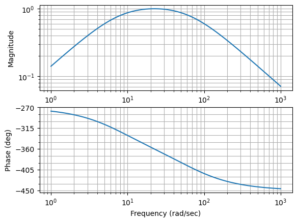
\[g(s)=\frac{71.43 s}{s^2 + 71.43 s + 502}\]To plot a bode diagramn, the command is not exactly the same like MATLAB. In this cas we need to use the bode_plot function.
h,ph,w=ct.bode_plot(g, plot='true')
The result, in this case, shows both the module and the phase response of the filter.
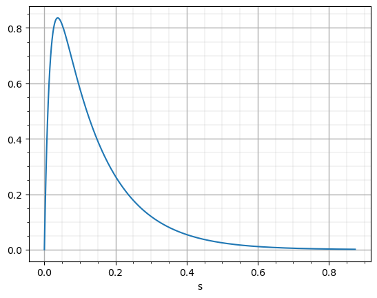
Even, with this library, we can check the step response of the filter. The function step_response returns us a time vector and a output vector that we can plot together to obtain the step reponse of the filter.
# Generate step response
T,y=ct.step_response(g)

# plot data
plt.plot(T,y)

plt.xlabel('s')

# plot grid
plt.grid(which = "major", linewidth = 1)
plt.grid(which = "minor", linewidth = 0.2)
plt.minorticks_on()
Now, if we need to discretize the transfer function, we can use the MATLAB command c2d
# discretizng filter
fSample = 50e3

gz=ct.c2d(g,1/fSample)
And also, the render of the equation is returned.
\[gz(z)=\frac{0.001428 z - 0.001428}{z^2 - 1.999 z + 0.9986}\quad dt = 2e-05\]To extract the numerator and the denominator of the transfer function variable, we can use the function tfdata, and it will return the numerator and the denominator vectors.
# Obtaining numerator and denominator
b,a=ct.tfdata(gz)
([[array([ 0.00142755, -0.00142755])]],
 [[array([ 1.        , -1.99857225,  0.99857245])]])
When we are working with embedded devices, installing MATLAB won’t be an option in every case. No one thinks about installing MATLAB in a Zynq MPSOC however, we already see that installing Python is possible and offers us great potential. In a design where we need a set of FIR or IIR filters, the implementation of the filters will be located on the FPGA and although often, the coefficients of these filters will be constants, in some situations we will need to modify the response of the filter also in real-time, either due to the tolerance of the components or because the system we are controlling has changed its response. In those cases, using Python, and libraries like Scipy and Control systems are the best option.


