Single pole filter without multiplications.
When I am working in a design for an FPGA, which involves the acquisition of any signal, I usually have to design a filter before using that signal in the control loop, or a protection. If the use of this signal is critical, like the mentioned before, I usually have to design a filter considering the position of the high power harmonics (switching harmonics mostly), the settling time of the filter if the filter is used on a signal that I use later for any kind of protection and obviously the aliasing. This set of requirements will mean that the filter cutoff frequency must be calculated, and implemented, with the least possible error.
In this case, does not matter if the filter uses 2, 4 or 8 MACC slices of the FPGA, because the task of this filter is relevant to the final process, but what if the filter is used in a signal that is not very relevant to the process? for example a temperature acquired with a noisy sensor, or any other signal with a large time constant which we have to filter out to avoid false measurements. For these cases we do not need an exact cutoff frequency, we just want to reduce the noise level to avoid, for example, false triggering faults. For these cases, the use of 2 MACC slices is not justified. For these cases we will need a filter that uses as less as possible the FPGA resources, even the response is not exact the desired one.
In this post I will show a single pole filter implementation, configured as low pass filter, without using MACC slices of the FPGA and a very low use of the resources. The filter used is based on the one that you can find in this post of DSPRelated.
First of all, we have to take a look to the single pole low pass filter equation:
\[H(s)=K \cdot \frac{1}{\tau s + 1}\]The differential equation of this filter is
\[\tau \cdot \frac{dy}{dt}=x-y\]being
\[\tau = \frac{1}{2\pi fc}\]The derivative component can be transformed to its equivalent discrete:
\[\tau \cdot \frac{\Delta y}{\Delta t} = x-y\]Now we can replace delta y by its equivalent and delta t by the sampling period of the filter, and the equation will looks like the above.
\[\tau \frac{y(t)-y(t-1)}{ts}=x(t)-y(t)\]Now, operating to isolate the term y(t), we will obtain the next equation.
\[y(t)=y(t-1)+(x(t)-y(t-1))\cdot \frac{ts}{\tau}\]At this point, we have a filter that uses additions, subtractions and a multiplication by a term. This term can be replaced by alpha, and the final equation will look like the next:
\[y(t)=y(t-1)+(x(t)-y(t-1)) \cdot \alpha\]Than the value of alpha is the division between the sampling time and tau is an pretty exact approximation when ts »> fc. In other cases the exact value of alpha will be:
\[\alpha = 1-e^{\frac{-ts}{\tau}}\]To simulate this filter in MATLAB, we have to define the filter parameters that will be the sampling frequency (100 ksps) and the cutoff frequency (50 Hz). The rest of the parameters will be obtain from these ones.
% Filter parameters

fs = 100e3;
fc = 50;

tau = 1/(2*pi*fc);
ts = 1/fs;
alpha = ts/tau;
%alpha = 1-exp(-ts/tau)
Now, since there is no s or z function that we can use the bode command, we will obtain the frequency response of the filter using a delta function. This delta function, that has a flat frequency spectrum, will be passed through the filter, and the fft of the filter’s output will be the frequency response. To generate the delta function we can use the next script.
% Signal
tmax = 0.8;

t = linspace(0,tmax,tmax*fs);
x = [1,zeros(1,length(t)-1)]; % delta function
Finally, the kernel of the filter is computed in a for loop.
y = zeros(length(t),1);

for i = [1:length(t)]
    if (i == 1)
        y(i) = 0 + alpha * (x(i)-0);
    else
        y(i) = y(i-1) + alpha * (x(i)-y(i-1));
    end
end
Then we have to compute the FFT of the output of the filter, and plot the result.
% fft
xfft = 20*log10(abs(fft(x)));
yfft = 20*log10(abs(fft(y)));

fVector = linspace(0,fs,length(t));

figure
semilogx(fVector, xfft)
xlim([0,fs/2])
hold on
semilogx(fVector, yfft)
xlim([0,fs/2])

legend('x','y')
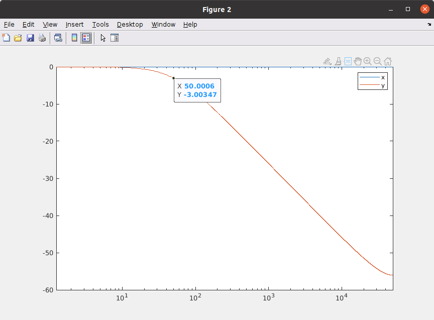
We can see how the cutoff frequency is 50 Hz as we have designed.
This filter has 1 multiplication, and the purpose of this post is a filter with no multiplications. To achieve this goal, we will replace the multiplication by a shift, but this has a cost. The value of alpha, when we replace the multiplication by a shift, is reduced to 1, 0.5, 0.25, 0.125, 0.06125… so the available cutoff frequencies is reduced considerably.
Let’s simulate it in MATLAB. This time, the configurable parameters of the filter are the sampling frequency and the value of the shift. Then we can do the reverse calculation to obtain the cutoff frequency.
% Filter parameters

fs = 100e3;
nshift = 8;

alpha = 2^(-nshift)
ts = 1/fs;
%tau = ts / alpha
tau = -ts/log(1-alpha)
wc = 1 / tau;
fc = wc/2/pi
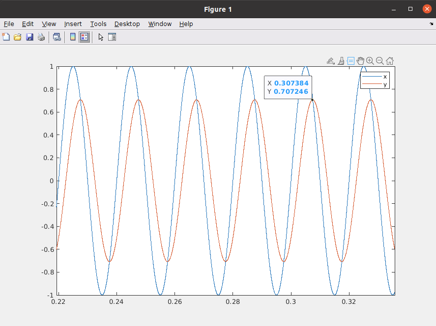
For a sampling frequency of 100 ksps and a shift of 8 positions, the resulting cutoff frequency is 66.16 Hz. If we pass through the filter a signal of that frequency, and an amplitude of 1, we will see how the output signal will be reduced by 0.707 (-3 dB).
To implement this filter in Verilog, first we have to configure through parameters the input and output widths, and also an internal width. The filter I have design has 2 AXI4 Stream interfaces for input and output data, so we will have to declare them in the ports list. Also, a input for the shift value will be added.
/**
  Module name:  axis_lpf_shifted_v1_0
  Author: P Trujillo ([email protected])
  Date: May 2021
  Description: Module to implement a 8th order FIR filter
  Revision: 1.0 Module created
**/

module axis_lpf_shifted_v1_0 #(
  parameter inout_width = 16,
  parameter inout_decimal_width = 15,
  parameter internal_width = 16,
  parameter internal_decimal_width = 15
  )(
  input aclk,
  input resetn,

  input [4:0] i5_alpha, /* alpha input in shift value */

  /* slave axis interface */
  input [inout_width-1:0] s_axis_tdata,
  input s_axis_tlast,
  input s_axis_tvalid,
  output s_axis_tready,

  /* master axis interface */
  output [inout_width-1:0] m_axis_tdata,
  output reg m_axis_tlast,
  output reg m_axis_tvalid,
  input m_axis_tready
  );

  localparam inout_integer_width = inout_width - inout_decimal_width; /* compute integer width */
  localparam internal_integer_width = internal_width - internal_decimal_width; /* compute integer width */

  wire signed [internal_width-1:0] input_int; /* input data internal size */
  reg signed [internal_width-1:0] reg_output_int; /* output internal size */

  /* resize signals to internal width */
  assign input_int = { {(internal_integer_width-inout_integer_width){s_axis_tdata[inout_width-1]}},
                            s_axis_tdata,
                            {(internal_decimal_width-inout_decimal_width){1'b0}} };

  /* tlast management */
  always @(posedge aclk)
    if (!resetn)
      m_axis_tlast <= 1'b0;
    else
      if (s_axis_tvalid)
        m_axis_tlast <= s_axis_tlast;

  /* tvalid management */
  always @(posedge aclk)
    if (!resetn)
      m_axis_tvalid <= 1'b0;
    else
      m_axis_tvalid <= s_axis_tvalid;

  /* filter kernel */
  always @(posedge aclk)
    if (!resetn)
      reg_output_int <= {inout_width{1'b0}};
    else
      if (s_axis_tvalid)
        reg_output_int <= reg_output_int + ((input_int - reg_output_int) >>> i5_alpha);

  /* resize for inout width */
  assign m_axis_tdata = reg_output_int >>> (internal_decimal_width-inout_decimal_width);


endmodule
Now, before the AXI4 Stream bus management, we can see a procedural block with the filter kernel, which is simply an addition and a subtraction, and the shift.
It is important to notice that if the subtraction input_int – reg_output_int is less than 2^i5_alpha, this term is zero, so this filter has an error in DC. This error can be eliminated by detecting the zero condition of this subtraction and adding directly the necessary amount, producing a zero error in DC.
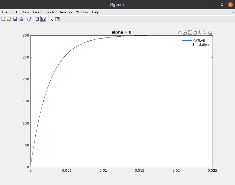
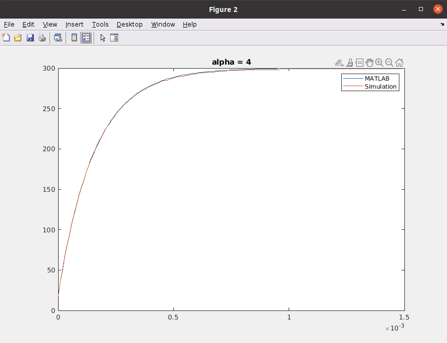
I have simulated the module for a 100 ksps sampling frequency and 2 values of shift, 8 and 4. Then a step signal has been used to check the output response and these are the results.
We can see how the response of the Verilog module is the same as the MATLAB output.
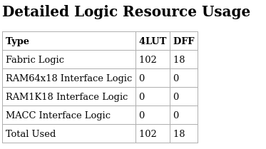
This filter has been implemented for an SmartFusion 2 SoC M2S010. The resources used by the filter are shown in the next table.
You can see that the filter is very cheap in terms of resources, but the cost is that the available cutoff frequencies are limited. We can improve the response by changing the sampling frequency, and always thinking in the aliasing. I think that it is an interesting Verilog module that we can add to our toolbox, and can get us out of trouble.
All the files are available on Github.


