Using MATLAB and FPGA-in-the-Loop to design a filter (Part 1)
If I say “a software for engineering”, most of you probably think on MATLAB. I don’t know if exist any engineering field which have not a package on MATLAB, and obviously, digital signal processing and FPGA design is not one of them. The package DSP System Toolbox will give us all the functions that we will need to design a filter or any processing system, Fixed-Point Designer allow us to quantize our processing system and verify the response on a digital system, and packages like HDL Coder or HDL Verifier will allow us to test our design in a real FPGA, and implement our system on our FPGA board.
On the next two posts, we are going to design a filter with the help of the Filter Designer tool. That filter will be quantified according the capabilities of our ADC. At this point we have to verify if the quantified model meets the defined criteria. Then, quantified filter will be simulated with a demo signal on Simulink. Next, we will generate the HDL code from de designed filter, and we will test this HDL with the real FPGA, but with our demo signal using FPGA-in-the-loop. This will give us information of the behavior of the filter on the real application. Finally, we will add the HDL of the filter in our Vivado Design, and we will test the integration of the filter with the rest of the design.
The application we are going to design is a decoder. It is very common to share the same transmission line to transfer different types of data, or even, to transfer power. The way to transfer data without interfering other kind of data, is to split transfers in different channels, but if only one channel is available, the way to do that is to split the frequency spectrum. That technique is used long time ago to transfer the sound of different radio stations through the same data line, the air. Other example is PLC (power line communication), where we can transfer power, at frequencies of 50Hz or 60Hz, and Ethernet data, at frequencies of hundreds of kHz. Once all data is transferred, we need to extract the range of frequencies that we have assigned, and discard the rest. To do that, we are going to design a band-pass filter.
The frequency spectrum of our transmission line is shown on the next figure. Each channel has a bandwidth of 20kHz, and the space between channels is 100kHz.

To avoid interference, we need to ensure at least –60dB on the others channels bandwidth. The filter we will design will obtain the signal on the channel 1 bandwidth, so the characteristics of the filter are:
| F(kHz) | dB |
|---|---|
| 910 | -60 |
| 990 | 0 |
| 1010 | 0 |
| 1090 | -60 |
(Use script signal_generation.m generates the line signals.)
To design the filter, first we will open Filter Designer tool.

With this tool we can configure all the characteristic of the filter. For this design, we will select a band-pass IIR Butterworth filter, with our frequency specifications. Once all the specification are correct, click on Design Filter and the filter response will be updated.

Once the filter is designed, we can export it to a workspace. To do that File > Export, and export it as an Object. On the next figure you can see the DFT of entire line data (red), and the response of the filter designed (blue). (Use the script filter_from_wks.m)

Once the filter is verified, the next is quantize the filter according out acquisition system. In this case, I will use the Eclypse Z7 board, and the ZMOD ADC. The output of the AD9648 has a maximum rate of 100 MSPS, but for this design a rate of 10 Msps is enough. The width of the output is 14 bits. With these parameters, we can configure the quantization by clicking on the button with the stairs.

Then select on filter arithmetic, and more option will be appearing. There are 3 tabs, one to configure the width of the coefficients, one for the width of the input and output, and the last to configure the width of the internal data of the filter.
Input and output widths have to be selected according the input and output data in our design. There is a very interesting option on the tool that allow to let MATLAB select the fractional part of the output to avoid overflow. In this case, if we select 14 bits on input and output, we will see that the fractional part of the output is reduced to 9. This will cause a loss of the resolution of the filter, and also means that output, in some point, can take values up to +-8 (3 bits). In my case, as the gain of the filter is 1, and for avoid base transformations on my FPGA design, I am going to select an output of 18 bits to keep the resolution of the output. We have to keep in mind this configuration, because in our design, we will have to add a saturation on the output of the filter.

Regarding the coefficients and the filter internals widths, if the response of the filter is acceptable, there is no need to change these parameters, but at this point you have to think on the part you will used on your design. In case of a Xilinx 7series part (Zynq7000, Artix7, Kintex7…), the DSP Slices DSP48E1 have a 25×18 bits multiplier (UG479), so to optimize the usage of this slices, the width of the coefficients, given the input is 14 bits, must be less than 25, but there is no problem in use larger widths, the synthesizer will use more than one slice for each multiplication.
With the quantization complete, we can check the quantified response of the filter, and it is very interesting check the position of the quantified poles to avoid instabilities. This step is very important when the filter designed has a large resonance on any point, because in this case, the poles are on the stability limit, and a poor quantization can make the filter unstable. Also, when we are designing an IIR filter, the quantization error turn more important as the order of the filter grows. To avoid that, IIR filters are designed as a group of 2nd order filters, or second order sections.
Once we have the filter designed and quantified, we can export this filter to a Simulink model by click on Realize Model.

Simulink window will open with the filter model added. Now, we can test the quantized model with the same signal we verified the continuous model. To do that we have to connect to the input of the filter a From Workspace block, and connect it to signal variable. At filter’s output we will add a To Workspace block to save data on workspace. Notice that the filter output is quantized, so we need to add a Convert module between the filter output and the To workspace block.

If we execute the model, and plot the signals, the result will show as follows:

At this point we have verified the continuous filter, and the quantized filter. On the next post we will generate the HDL of the filter, and test it using FPGA-in-the-loop and Eclypse Z7 board. Last, we will generate a block design with the filter and we will test it with a real application.
All code scripts are available on Github and FileExchange.