Implementing a Single-Precision Floating-Point Biquad on Versal
 ig-g57d
In my daily work, y I often need to implement digital filters on FPGAs, and since I usually work with 7 Series FPGA, all my filters are designed using fixed-point arithmetic. Is true that I can implement floating-point arithmetic using those FPGAs, but it would be an overkill in terms of resources and complexity. On the other side, working with fixed-point arithmetic needs a lot of care about the overflows. Usually, this is not a big issue when you have been working with fixed-point for years, and know exactly all the ranges of your signals, however, there is another problem that needs more attention, the quantization.
For filters, or systems in general, with very small parameters, you need to use a lot of bits to represent those parameters, in addition, if this small parameters are in the same system than other large parameters, the size of the signals becomes a problem. One solution for this problem is using floating-point arithmetic.
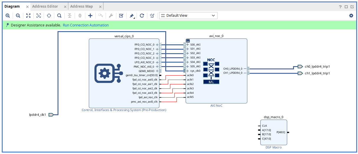
In a previous post I introduced the iWave Global iG-G57D board, based on the Versal AI Edge VE2302, and I went through the CIPS, the AXI NoC and a simple AXI4-Lite peripheral. This time I want to go deeper into the programmable logic and use one of the features that made me want to try Versal in the first place: the DSP58 slices and their native floating-point support.
The example I chose is a biquad, the second-order IIR section that is the building block of almost every audio and control filter. Implementing it in fixed point is the classic approach, but Versal lets us stay in single-precision floating point end to end, which is much more comfortable when you port a filter design straight from MATLAB or from a control model. In this article I want to show you how to instantiate a floating-point multiply-accumulate on Versal, how to chain five of them to build the biquad, and how to integrate the resulting IP in a block design with the NoC.
Table of contents
- The biquad as a chain of MACC operations
- Floating point on Versal: the DSP58
- Instantiating a floating-point MACC
- Configuring the Floating-Point IP
- Building the biquad with five chained MACCs
- Integrating the IP in the block design
- Verifying with VIO and ILA
- Fixing the clock and reset critical warning
- Conclusions
The biquad as a chain of MACC operations
A biquad is a second-order IIR filter, and as any IIR filter it is built entirely out of multiply-and-accumulate operations. Its direct-form I difference equation is:
\[y(k) = x(k-2) \cdot b2 + x(k-1) \cdot b1 + x(k) \cdot b0 - y(k-2) \cdot a2 - y(k-1) \cdot a1\]So computing one output sample takes five multiplications and the accumulation of all the products. This is exactly the kind of work a DSP slice is built for, and it tells us right away what the datapath should look like: a chain of MACC units, each one taking a coefficient, a delayed sample, and the partial result coming from the previous stage.
The only subtlety is the sign of the feedback terms. The a1 and a2 coefficients are subtracted from the output, but to keep every stage identical I implemented a single MACC core that always computes A*B + C. To make the subtraction work without a dedicated subtractor, the user simply feeds the a1 and a2 coefficients already negated, and the chain stays homogeneous.
Floating point on Versal: the DSP58
A biquad needs a device that is good at MACC operations. In a DSP or a microcontroller those operations live in the floating-point unit; in Versal they live in the DSP58 slices. The DSP58 is the newest generation of AMD DSP slices and, unlike the DSP48 in previous families, it can perform floating-point MACC operations natively, in single precision, without building the floating-point datapath out of fabric and extra multipliers.
That is the feature I wanted to exploit here. Instead of quantizing the filter to fixed point, choosing word lengths and worrying about overflow in the accumulator, I can keep the whole biquad in single-precision floating point and let the DSP58 do the heavy lifting.
Instantiating a floating-point MACC
There are three ways to get a DSP58 into your design, and only one of them is really convenient for floating point.
The first one is to drop a DSP block directly from the block design. This is the most visual option, but it does not let you configure the slice for floating-point operation, so it is a dead end for our purpose.
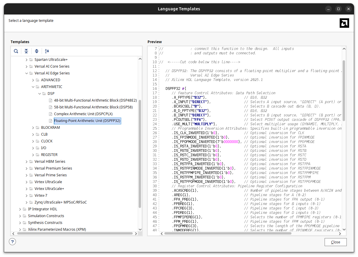
The second option is to use the Language Templates, under Verilog > Device Primitive Instantiation > Versal AI Edge > ARITHMETIC > DSP. This gives you the raw primitive, but it has the obvious drawback that you have to configure every single parameter of the DSP58 by hand, which is error-prone and tedious.
The best option is the IP Catalog, under Vivado Repository > DSP and Math > General > Floating Point. This IP wraps the DSP58 in floating-point mode and exposes a clean AXI4-Stream interface, so you get the native floating-point MACC without touching low-level parameters.
Configuring the Floating-Point IP
In the first tab we select the operation. For a biquad we want Unfused Multiply-Add.
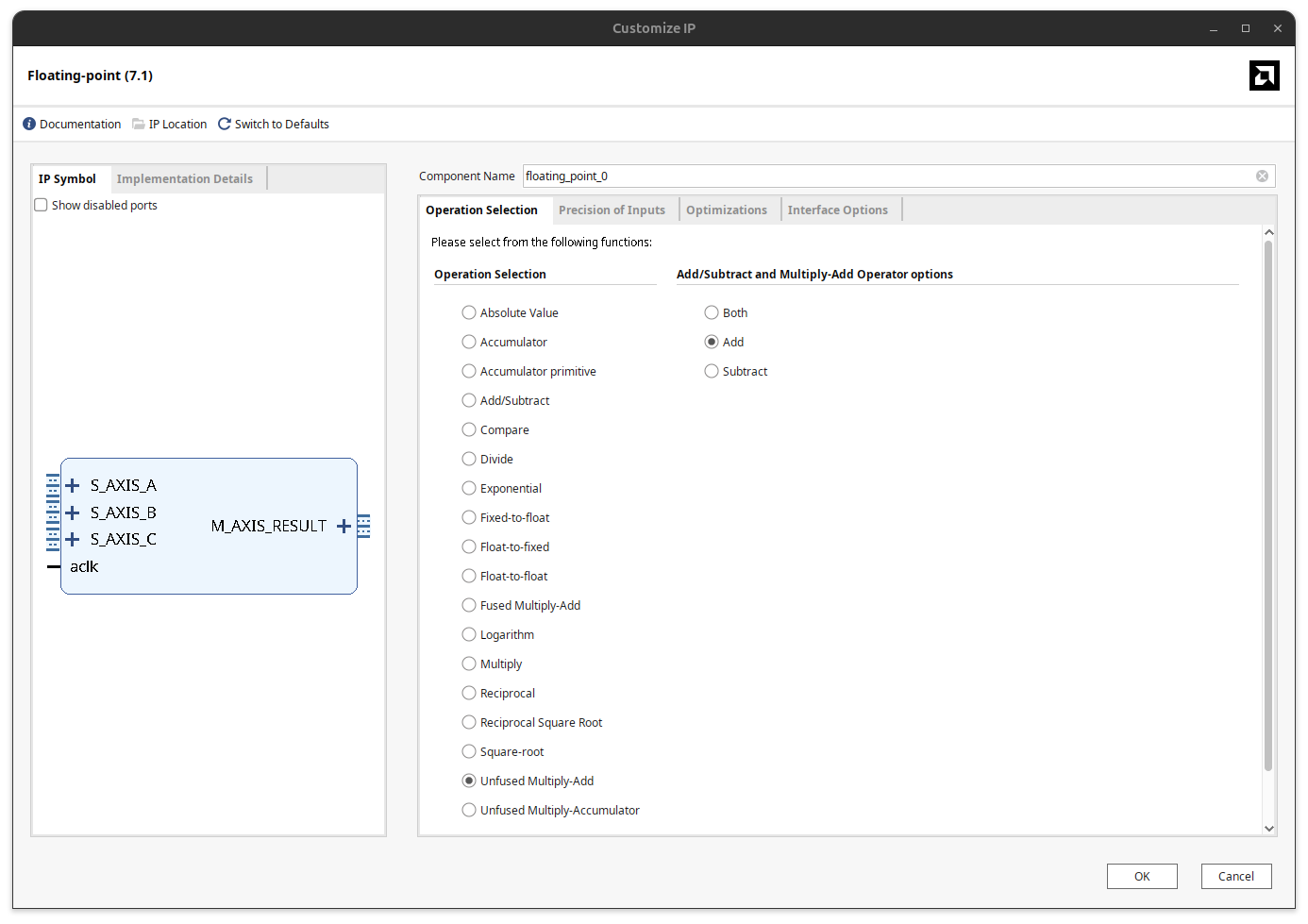
The difference between Multiply-Add and Multiply-Accumulator is that the Add variant has an extra input for the addend, while the Accumulator only accumulates onto its own internal result. The Add variant is exactly what we need, because each stage of the biquad has to add the partial result coming from the previous MACC.
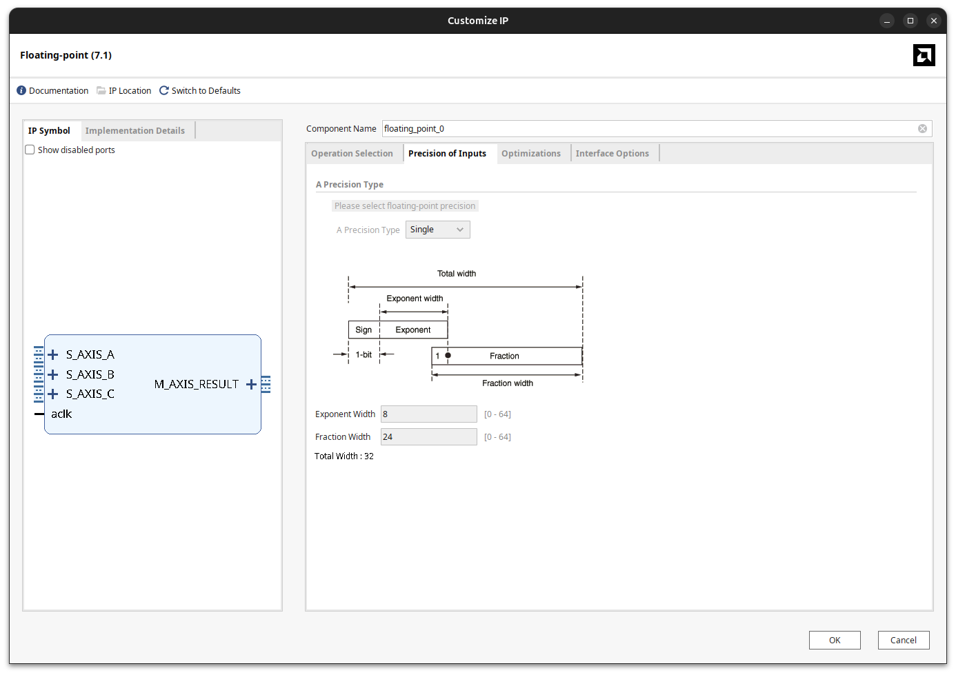
Once Multiply-Add is selected, the next tab forces us to work in single precision.
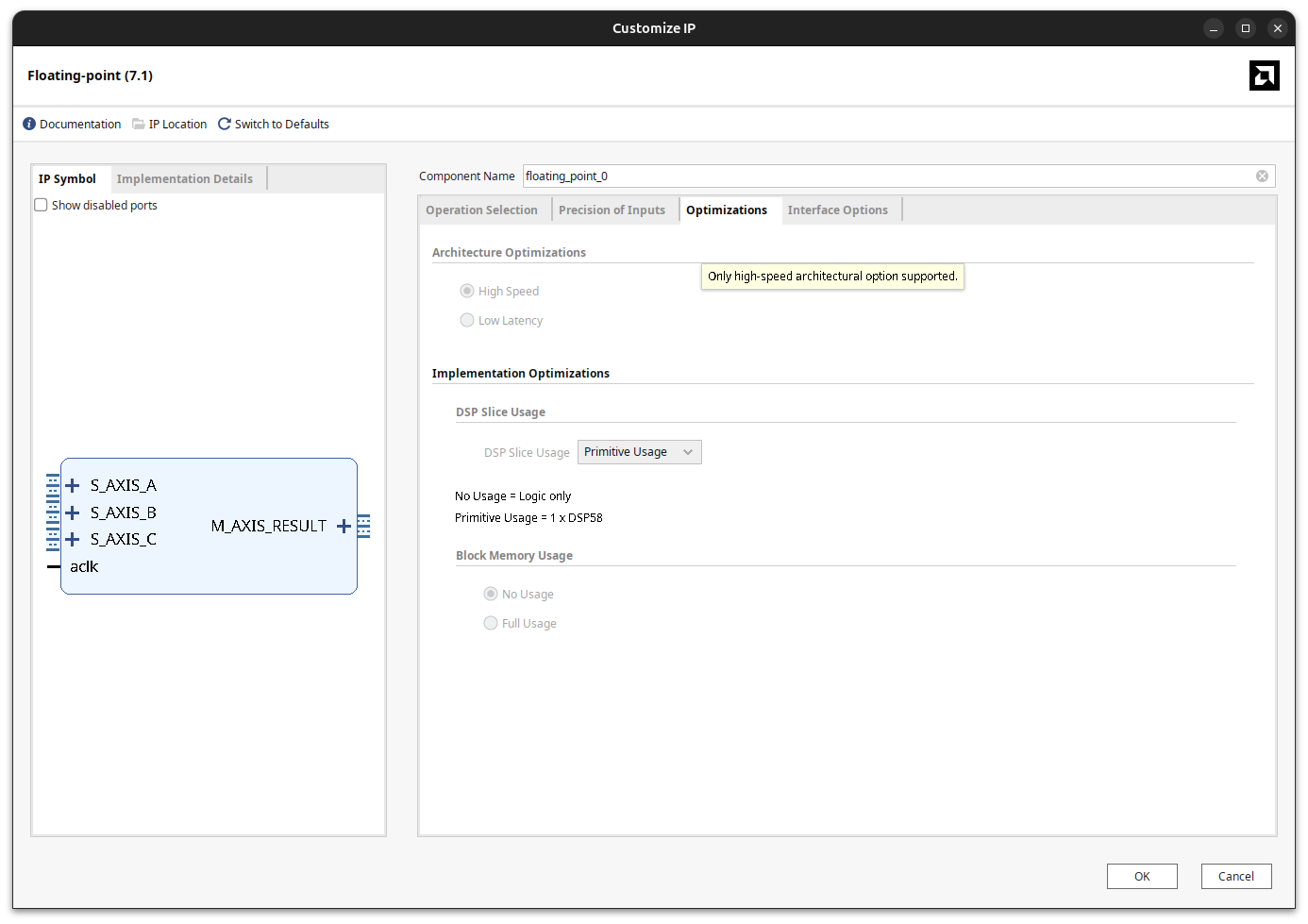
The third tab is completely locked and forces the IP to use the DSP58 primitive, which is precisely what we are after.
The last tab exposes some interface options and, more importantly, the latency. The latency is just the number of internal registers we enable inside the DSP58 primitive. The right value depends on the clock frequency you want to reach: the higher the frequency, the more pipeline registers you need. By default it is set to Use Maximum Latency, which configures 5 internal registers.
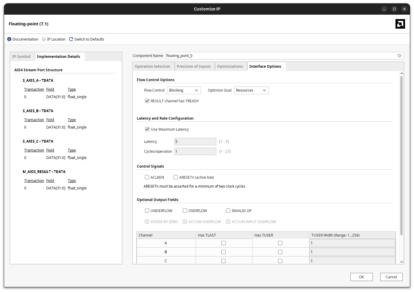
The Optimize Goal parameter is worth a comment. With Resources the IP lets you bring the number of pipeline registers down to 1, trading throughput for area and latency. With Performance the IP is configured to reach the maximum clock frequency, so the minimum number of pipeline registers goes up to 3 and the maximum goes from 5 to 7. In the implementation details you can also see that the IP creates three slave AXI4-Stream interfaces (one for each operand, A, B and C) and one master AXI4-Stream interface for the result.
When the configuration is done you can generate the IP outputs and keep just the .xci file, which lives in the project under versal_iir.srcs > ip > fp32_macc, together with the instantiation template:
fp32_macc your_instance_name (
  .aclk(aclk),                                  // input wire aclk
  .s_axis_a_tvalid(s_axis_a_tvalid),            // input wire s_axis_a_tvalid
  .s_axis_a_tready(s_axis_a_tready),            // output wire s_axis_a_tready
  .s_axis_a_tdata(s_axis_a_tdata),              // input wire [31 : 0] s_axis_a_tdata
  .s_axis_b_tvalid(s_axis_b_tvalid),            // input wire s_axis_b_tvalid
  .s_axis_b_tready(s_axis_b_tready),            // output wire s_axis_b_tready
  .s_axis_b_tdata(s_axis_b_tdata),              // input wire [31 : 0] s_axis_b_tdata
  .s_axis_c_tvalid(s_axis_c_tvalid),            // input wire s_axis_c_tvalid
  .s_axis_c_tready(s_axis_c_tready),            // output wire s_axis_c_tready
  .s_axis_c_tdata(s_axis_c_tdata),              // input wire [31 : 0] s_axis_c_tdata
  .m_axis_result_tvalid(m_axis_result_tvalid),  // output wire m_axis_result_tvalid
  .m_axis_result_tready(m_axis_result_tready),  // input wire m_axis_result_tready
  .m_axis_result_tdata(m_axis_result_tdata)     // output wire [31 : 0] m_axis_result_tdata
);
Building the biquad with five chained MACCs
The biquad needs five MACC operations, and we want them chained so the partial result flows from one DSP58 to the next through the dedicated PCIN and PCOUT cascade paths. Because of this chaining the operations cannot run in parallel: even though we use five DSP58 blocks, the total latency is 5 cycles per block times 5 blocks, that is 25 clock cycles. This number can be reduced if we lower the number of pipeline registers per MACC, at the cost of maximum clock frequency.
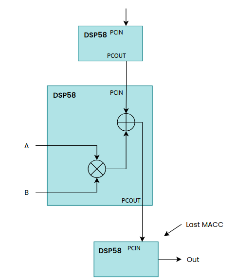
To keep the design uniform I instantiate a single fp32_macc core five times, and every instance computes the same A*B + C operation. The first stage seeds the chain with the feedforward term b0 * x[n] plus a floating-point zero, and each subsequent stage adds its own product to the running result coming from the previous stage. The feedback stages use the negated a1 and a2 coefficients, so the subtraction in the difference equation happens naturally:
/* MAC0: result = b0 * x[n] + 0.0 */
fp32_macc u_mac0 (
.aclk(aclk),
.s_axis_a_tvalid(ce),
.s_axis_a_tready(mac0_a_tready),
.s_axis_a_tdata(coeff_b0),
.s_axis_b_tvalid(ce),
.s_axis_b_tready(mac0_b_tready),
.s_axis_b_tdata(x_in),
.s_axis_c_tvalid(ce),
.s_axis_c_tready(mac0_c_tready),
.s_axis_c_tdata(FP32_ZERO),
.m_axis_result_tvalid(mac0_result_tvalid),
.m_axis_result_tready(1'b1),
.m_axis_result_tdata(mac0_result_tdata)
);

/* MAC1: result = b1 * x[n-1] + mac0_result */
fp32_macc u_mac1 (
.aclk(aclk),
.s_axis_a_tvalid(mac0_result_tvalid),
.s_axis_a_tready(mac1_a_tready),
.s_axis_a_tdata(coeff_b1),
.s_axis_b_tvalid(mac0_result_tvalid),
.s_axis_b_tready(mac1_b_tready),
.s_axis_b_tdata(x_prev1),
.s_axis_c_tvalid(mac0_result_tvalid),
.s_axis_c_tready(mac1_c_tready),
.s_axis_c_tdata(mac0_result_tdata),
.m_axis_result_tvalid(mac1_result_tvalid),
.m_axis_result_tready(1'b1),
.m_axis_result_tdata(mac1_result_tdata)
);

/* MAC2: result = b2 * x[n-2] + mac1_result */
fp32_macc u_mac2 (
.aclk(aclk),
.s_axis_a_tvalid(mac1_result_tvalid),
.s_axis_a_tready(mac2_a_tready),
.s_axis_a_tdata(coeff_b2),
.s_axis_b_tvalid(mac1_result_tvalid),
.s_axis_b_tready(mac2_b_tready),
.s_axis_b_tdata(x_prev2),
.s_axis_c_tvalid(mac1_result_tvalid),
.s_axis_c_tready(mac2_c_tready),
.s_axis_c_tdata(mac1_result_tdata),
.m_axis_result_tvalid(mac2_result_tvalid),
.m_axis_result_tready(1'b1),
.m_axis_result_tdata(mac2_result_tdata)
);

/* MAC3: result = coeff_a1 * y[n-1] + mac2_result */
fp32_macc u_mac3 (
.aclk(aclk),
.s_axis_a_tvalid(mac2_result_tvalid),
.s_axis_a_tready(mac3_a_tready),
.s_axis_a_tdata(coeff_a1),
.s_axis_b_tvalid(mac2_result_tvalid),
.s_axis_b_tready(mac3_b_tready),
.s_axis_b_tdata(y_prev1),
.s_axis_c_tvalid(mac2_result_tvalid),
.s_axis_c_tready(mac3_c_tready),
.s_axis_c_tdata(mac2_result_tdata),
.m_axis_result_tvalid(mac3_result_tvalid),
.m_axis_result_tready(1'b1),
.m_axis_result_tdata(mac3_result_tdata)
);

/* MAC4: result = coeff_a2 * y[n-2] + mac3_result */
fp32_macc u_mac4 (
.aclk(aclk),
.s_axis_a_tvalid(mac3_result_tvalid),
.s_axis_a_tready(mac4_a_tready),
.s_axis_a_tdata(coeff_a2),
.s_axis_b_tvalid(mac3_result_tvalid),
.s_axis_b_tready(mac4_b_tready),
.s_axis_b_tdata(y_prev2),
.s_axis_c_tvalid(mac3_result_tvalid),
.s_axis_c_tready(mac4_c_tready),
.s_axis_c_tdata(mac3_result_tdata),
.m_axis_result_tvalid(mac4_result_tvalid),
.m_axis_result_tready(1'b1),
.m_axis_result_tdata(mac4_result_tdata)
);
The output of u_mac4 is the filtered sample y[n], which is then fed back into the y_prev1 and y_prev2 registers for the next iteration.
Integrating the IP in the block design
With the peripheral created, the next step is to give it access to the rest of the system. In the block design I add an AXI master on the NoC, connected to the PL.
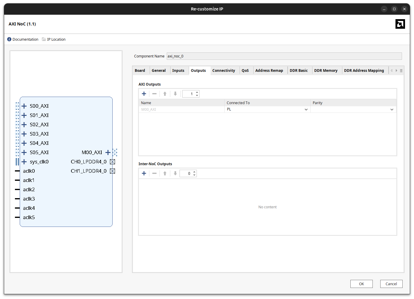
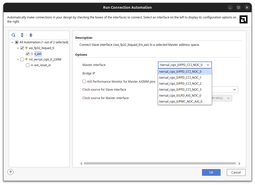
Once the master exists, it has to be routed to one of the slaves. This is done from the Connectivity tab of the NoC.
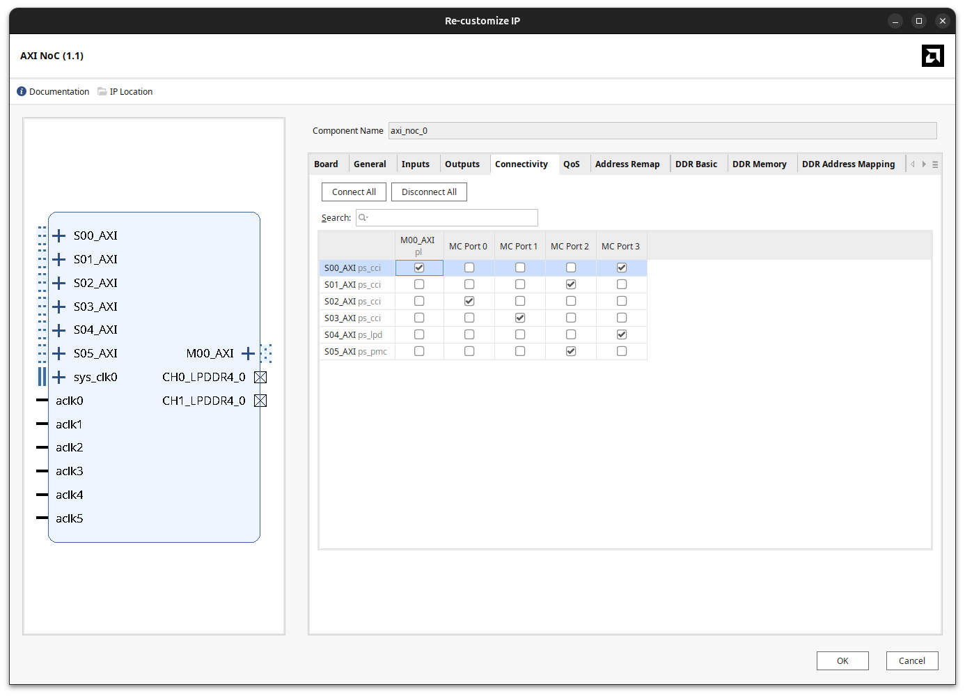
There is a detail here that can be confusing the first time. After the NoC master is connected to a slave and our new IP is added, the master interface selection does not show the NoC master. Instead, it shows directly the CIPS master that the NoC master is connected to, and it tells us that it will use /axi_noc_0 as a bridge.
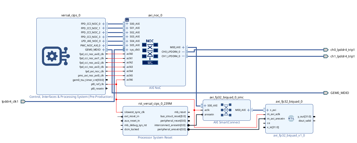
Once everything is wired, the block design looks like this.
Verifying with VIO and ILA
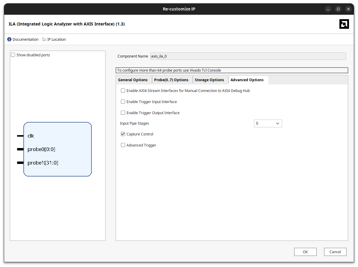
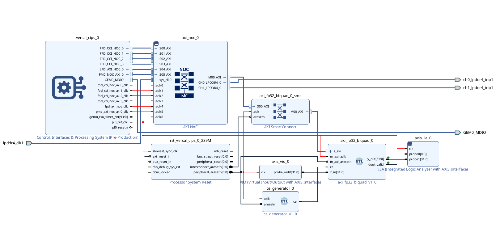
To check that everything works, I added an axis_vio so I can drive the filter input from JTAG, and an axis_ila to observe the output. In the axis_ila configuration it is important to enable the Capture Control tick, because that way we can capture only on the edges of the dout_valid signal instead of filling the buffer with idle samples.
The complete block design, now including the debug cores, looks like this.
Fixing the clock and reset critical warning
When I validated this design, Vivado raised a critical warning saying that the clock connected to the biquad IP was not the same as the one connected to the AXI Interconnect, which is not actually true. You can live with this critical warning, or you can get rid of it by adding the interface attributes to the clock and reset inputs. These attributes tell Vivado that the clock and reset belong to the AXI4-Lite interface:
(* X_INTERFACE_INFO = "xilinx.com:signal:clock:1.0 m_axi_aclk CLK" *)
(* X_INTERFACE_PARAMETER = "XIL_INTERFACENAME m_axi_aclk, ASSOCIATED_BUSIF s_axi, ASSOCIATED_RESET m_axi_aresetn" *)
input m_axi_aclk,

(* X_INTERFACE_INFO = "xilinx.com:signal:reset:1.0 m_axi_aresetn RST" *)
(* X_INTERFACE_PARAMETER = "XIL_INTERFACENAME m_axi_aresetn, POLARITY ACTIVE_LOW" *)
input m_axi_aresetn,
After adding these attributes the validation no longer reports any warning or error. Keep in mind that, at this point, we are adding Vivado-specific attributes, so our IP stops being compatible with other tools like Quartus. This could be guarded with an `ifdef XILINX_VIVADO around the attributes, but in this particular case the IP already uses Versal-specific primitives, so it is not portable to, for example, an Agilex 3 anyway.
Conclusions
Some years ago (many maybe), floating point was something that you only found in high-end processors, and I have to say that what game developers did using just fixed-point and imagination was amazing. Nowadays, the Floating-Point Units (FPU) are a kind of commodity in the CPU and MCU world, however, in the FPGA world only a few families include it (except for Agilex, that is even more difficlt to find a part without native floating-point support). The AMD Versal ACAP is one of those families, and the DSP58 slices are the one in charge of this task.
Will this be a game-changer for FPGA-based DSP? I don`t think so, at least for now. Even LLM uses fixed-point quantizations to improve the performance, so for most applications fixed-point is still the way to go. However, for some specific use cases like audio filters or control loops, where the coefficients can be very small and the quantization can cause stability problems, having native floating-point support in the fabric is a great advantage. It allows you to implement your filter directly in floating point without worrying about quantization and overflow, and it makes the design process much more straightforward.
But wait a minute, that does not mean thay now, you can implement MATLAB code directly on Versal, you still need to know very well what are you doing, and how to map your algorithm to the hardware. The DSP58 slices are powerful, but they are not magic, and you still need to design your datapath and control logic carefully to get the best performance out of them.